Project Description
Key Contributions
- Developed a framework for contextualizing visual data through textual descriptions by identifying actions in scenes and modeling relationships between subjects and objects.
- Collaborated with cross-industry, multi-partner teams, including Microsoft Media Group, on video analysis and image processing research.
- Participated in regular meetings with the industry partner (Microsoft Media Group) to align project goals with their needs and communicate our capabilities.
- Attended weekly project meetings to present progress, exchange ideas, and provide feedback to other research teams.
- Evaluated and refined the MoE-VRD architecture and implementation for improved scene understanding.
- Reviewed experimental design and reported key findings.
- Led major revisions and served as the corresponding author, rewriting the article and presentation for publication.
- Conducted a comprehensive literature review to strengthen the research context and support dissemination.
Tools & Technologies
- Python, PyTorch, TensorFlow, Pandas, NumPy, Torchvision
- OpenCV, scikit-learn, PIL (Pillow)
- Matplotlib (mpl_toolkits), Seaborn, Plotly
Code / Git
Research / Paper
Presentation
- Microsoft Media group & Dept. of Systems Design Engineering, University of Waterloo
Additional Context
Video Relationship Detection
In this section, I will explain the fundamentals of the video relationship detection approach utilized in our model architecture.
Problem Formulation
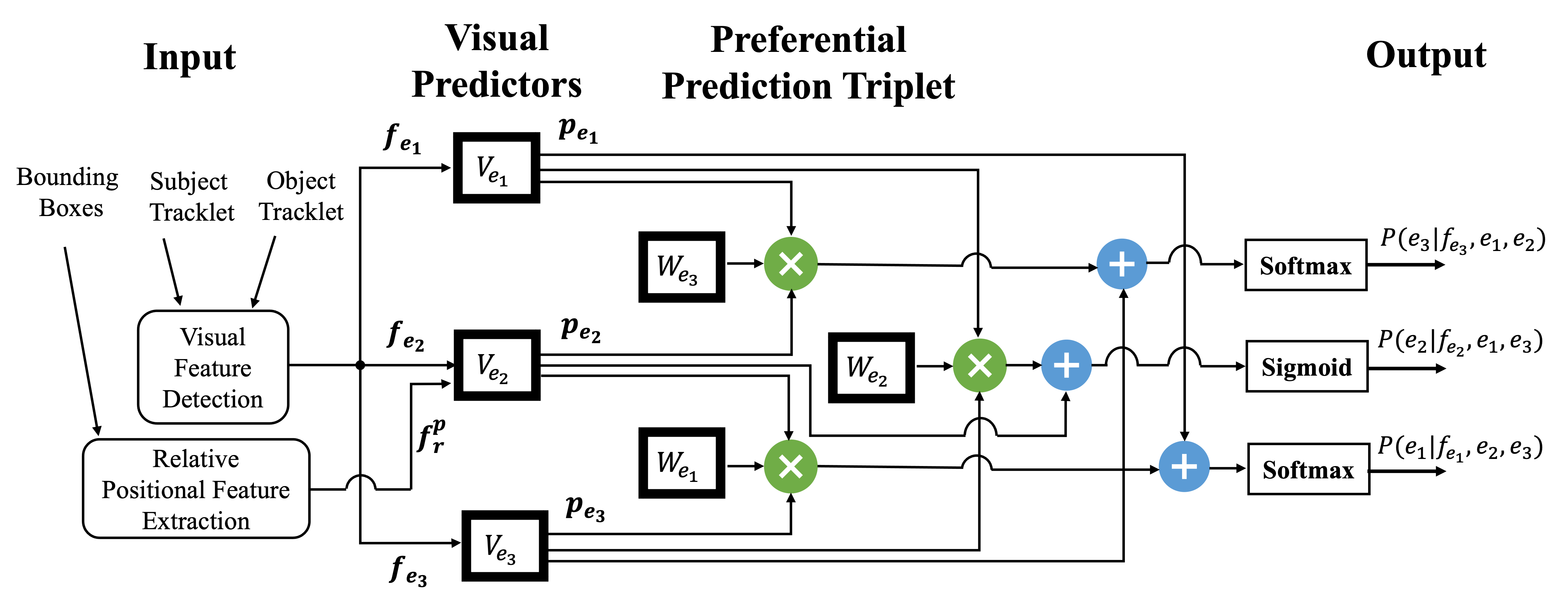
Assume a set of three entities \( \mathbb{E} = \{e_1, e_2, e_3\} \), which represent Subject \(e_1\), predicate \(e_2\), and object \(e_3\), with their corresponding features \( \mathbb{F} = \{f_{e_1}, f_{e_2}, f_{e_3}\} \) to build the language triplet \( < \text{subject}, \text{predicate}, \text{object}>\). We model the problem of video visual relationship detection as the joint probability of:
\( \text{P}(< e_1, e_2, e_3 > | < f_{e_1}, f_{e_2}, f_{e_3} >) \),
where we factorized this joint probability as follows:
\( \text{P}(e_1| f_{e_1}, e_2, e_3) \cdot \text{P}(e_2| f_{e_2}, e_1, e_3) \cdot \text{P}(e_3| f_{e_3}, e_1, e_2) \),
to aid in inference time when there is ambiguous visual information, since the classes of any two components imply a preference over the class of the third. Each of these three conditional probabilities is modelled by a classifier consisting of a visual predictor and a preferential predictor.
The visual predictor is a deep neural network, which learns visual patterns of the subject, predicate, and object. The preferential predictor applies learnable dependency tensors to refine the prediction of one variable conditioned on the values of the other two:
\[ e_{pr} = \left\{ \begin{aligned} \text{P}(e_1| f_{e_1}, e_2, e_3) &= \Phi (\text{V}_{e_1} \cdot f_{e_1}) + p_{e_2} \cdot \text{W}_{e_1} \cdot p_{e_3} \\ \text{P}(e_2| f_{e_2}, e_1, e_3) &= \Phi (\text{V}_{e_2} \cdot f_{e_2}) + p_{e_1} \cdot \text{W}_{e_2} \cdot p_{e_3} \\ \text{P}(e_3| f_{e_3}, e_1, e_2) &= \Phi (\text{V}_{e_3} \cdot f_{e_3}) + p_{e_1} \cdot \text{W}_{e_3} \cdot p_{e_2} \end{aligned} \right\} \]
where \(\text{V}_{e_1}\), \(\text{V}_{e_2}\), and \(\text{V}_{e_3}\) are the learnable weights of the visual predictors. In our case study, the weights of the subject and object classifiers are shared, thus \(\text{V}_{e_1} = \text{V}_{e_2}\). On the other hand, for preferential prediction \(\text{W}_{e_1}\), \(\text{W}_{e_2}\), and \(\text{W}_{e_3}\) model the dependency of one class over the other two, separately parametrized for each classifier. \(\Phi\) represents the nonlinear activation, here implemented by a \(\text{Softmax}\) function for the subject and object classes, and a \(\text{Sigmoid}\) function for the predicate class.
Sparsely Gated Mixture-of-Experts
Our MoE-VRD The MoE consists of a set of N expert networks \(\text{E}_1, \text{E}_2, ..., \text{E}_N\) and one gating network, G, whose output is a sparse binary N -dimensional vector. The experts are themselves identical feed-forward neural networks, each with their own parameters.
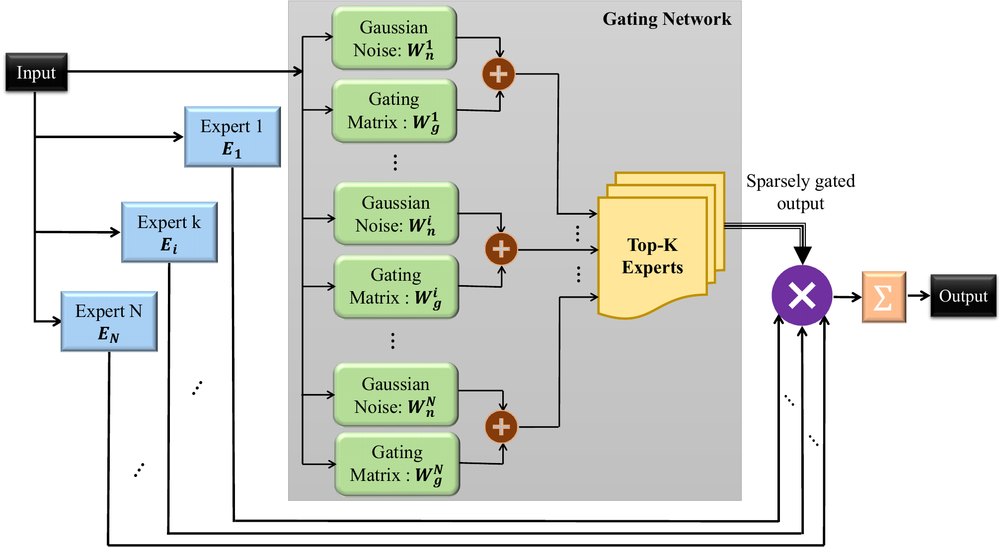
Given an input \(x\), the output of the ith expert’s function is denoted as \(E_i(x)\). These N outputs are combined in the MoE layer as:
\( y = \sum_{i=1}^{N} G(x)_i \cdot E_i(x) \),
where \(G(x)_i\) represents the output of the gating network. The sparsity in computation, one of the key strengths of the MoE approach, is realized by the explicit sparsity of the gating output:
\( G(x)_i = 0 \quad \text{for most} \quad i \),
where if \( G(x)_i = 0 \) the corresponding expert is eliminated from learning procedure.
We adopt a single–layer gating function:
\[ G(x)_i = \text{Softmax}\left( {\text{top}_{K}} \left( \text{W}^{i}_{g} \cdot x + N_g (\text{W}^{i}_{n} \cdot x) \right) \right), \]
where \(\text{top}_K\) selects the K largest values (the best experts), and \(\text{W}^{i}_{g}\) and \(\text{W}^{i}_{n}\) are trainable gating and noise weight matrices, respectively, which are parametrized for each expert i. Since the number of samples sent to the gating layer is discrete, and therefore not applicable to back-propagation, the inclusion of the noise term Ng (x) allows for a smooth estimate of the number of samples used for each expert in each batch, thus allowing for the back-propagation of gradients.
The noise function is defined as:
\[ \text{N}_g (x) = \text{StandardNormal}() · \text{Softplus}(x), \quad \text{where} \quad \text{Softplus}(x) = \frac{1}{\beta} \text{log}(1 + \beta x) \]
where \(\text{Softplus}\) is a smooth approximation of the \(\text{ReLU}\) function to constrain the output to be positive.
Moreover, an importance term is considered in the overall loss to address imbalances resulting from the self-reinforcing effect Lu et. al (2021), which occurs when certain favoured experts are trained more rapidly and thus are selected even more by the gating network.
The importance loss is calculated as follows:
\[ L_{\text{importance}} (x) = \alpha \left( \text{CV}(g) + \text{CV}(l) \right), \]
where \(\alpha\) is a hand-tuned scaling factor, g is the batch-wise sum of gate values (over batch B):
\[ g = \sum_{x\in B} G(x). \]
The load \(l\) the load, summed over the positive gate values is computed as:
\[ l = \sum_{x\in B, g>0} G(x), \]
Finally, we applied \(\text{CV}(·)\), the coefficient of variation:
\[ \text{CV} = \frac{\text{var}(x)}{\text{mean}(x)^2 + \epsilon}, \]
to encourage experts to have a more balanced (equal) importance.Video Relationship Detection Using Mixture-of-Experts
Finally, we have the full model architecture of MoE-VRD.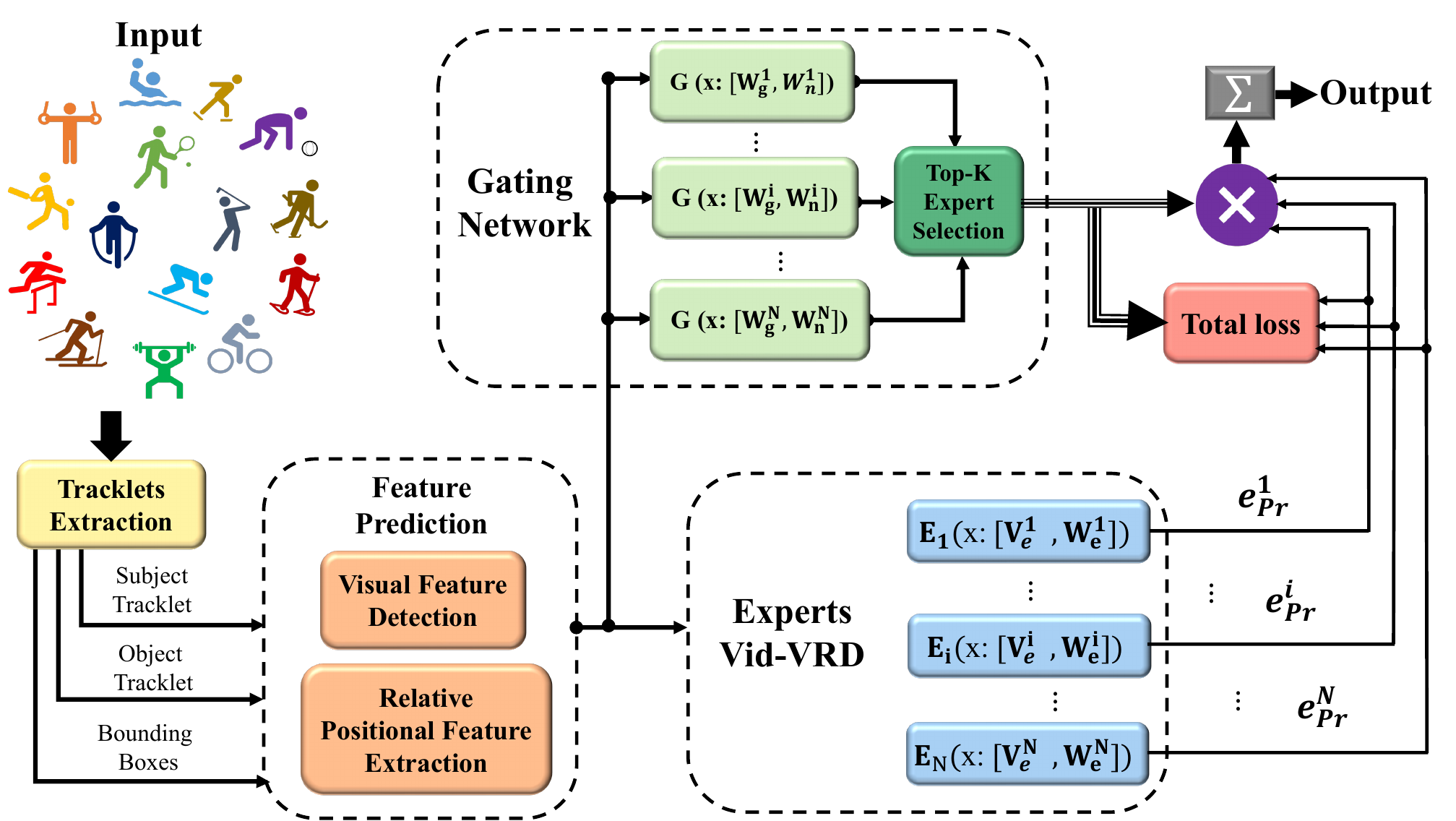
Object Tracklet Proposals
We employ Seq-NMS Han et. al (2016) to generate object tracklet proposals as a pre-processing step for the relational classifier experts. For frame-level object detection, we use a Faster-RCNN with an Inception-ResNet backbone Szegedy, et. al (2017), pretrained on the Open Images dataset, providing a robust, generic object detector. Bounding boxes and corresponding region features are then extracted, and Seq-NMS compacts these into a set of object tracklets that serve as inputs to the expert neural networks.
Feature Extraction
Applying the object tracklet proposals, we generate two types of features: Visual Features and Relative Positional Features.
Visual Features
To generate the visual features \(f\), the bounding boxes are applied to extract the pretrained deep visual features of the subject and object entities, and the predicate’s visual feature is computed through a concatenation of the subject and object visual feature vectors.
Relative Positional Features
We extract a relative positional feature to represent the spatio-temporal relationship between the entities. For each pair of object tracklets, the algorithm computes the relative distance between the subject and object by encoding the spatial and temporal relative positional feature:
\[ f^{p}_{r} = \left[ \frac{x^{p}_{e_1}-x^{p}_{e_3}}{x^{p}_{e_3}}, \frac{y^{p}_{e_1}-y^{p}_{e_3}}{y^{p}_{e_3}}, \text{log}\frac{w^{p}_{e_1}}{w^{p}_{e_3}}, \text{log}\frac{h^{p}_{e_1}}{h^{p}_{e_3}}, \text{log}\frac{w^{p}_{e_1} h^{p}_{e_1}}{w^{p}_{e_3} h^{p}_{e_3}}, \frac{t^{p}_{e_1}-t^{p}_{e_3}}{30} \right], \]
where \(p \in [b, e]\) represents the beginning or ending bounding box, characterized by coordinates \((x, y)\), width \(w\), height \(h\), and time \(t\) for subject \(e_1\) and object \(e_3\) . A feed-forward network is used to fuse the subject’s and object’s visual features \(f_{e_1}\) , \(f_{e_3}\) with the relative positional features of the beginning and ending bounding boxes \(f^{b}_r\) , \(f^{e}_r\) , where the relative positional feature \(f^{p}_r\) provides the expert with additional information to recognize visual relationships.
In summary, each encapsulated expert consists of an object predictor, a subject predictor, and a predicate predictor — each of which is a basic feed-forward network, allowing for a set of modestly-sized, nimble experts to speed up training and inference, when compared to an equivalent single monolithic network.
Experiments and Results
Datasets
We used two VidVRD benchmark datasets:
- ImageNet-VidVRD Shang et. al (2017): is the first dataset for video visual relation detection. It consists of 1,000 videos, which are manually annotated with video relation instances.
- VidOR Shang et. al (2019): is a recently-released large-scale benchmark, which contains 10,000 social media videos.
Evaluation Metrics
In object detection, two key tasks must be addressed: localization and classification. Localization involves determining the precise position of an object, such as its bounding box, while classification identifies the object’s category or type.
In object detection, precision and recall are typically calculated using a specified Intersection over Union (IoU) threshold, which quantifies the overlap between predicted and actual bounding boxes. When the IoU for a predicted bounding box exceeds this threshold, the prediction is classified as a true positive; otherwise, it is a false positive. Metrics such as Recall@50 evaluate recall at an IoU threshold of 50%, permitting bounding boxes to overlap by at least 50%. Other metrics, like Recall@100 and Precision@10, are similarly defined based on their respective thresholds.
To evaluate how well the mixture of experts detects ground truth relation instances in each test video, we use two types of metrics: relation tagging and relation detection.
- Relation tagging assesses the precision of detected relation triplets without considering their spatio-temporal accuracy. This metric simply checks if the relation was detected, ignoring precise timing or spatial details. Tagging performance is measured by Precision@1 (P@1), Precision@5 (P@5), and Precision@10 (P@10).
- Relation detection, on the other hand, considers both the relation triplet and the trajectories of the subject and object. A detected relation instance is only correct if it matches the ground-truth relation instance and the volumetric Intersection-over-Union (vIoU) of both subject and object trajectories exceeds a threshold of 50%. This performance is quantified using Mean Average Precision (mAP), Recall@50 (R@50), and Recall@100 (R@100).
All experiments are repeated ten times with varied random seeds for each expert, and we report the mean and standard deviation scores for each metric.
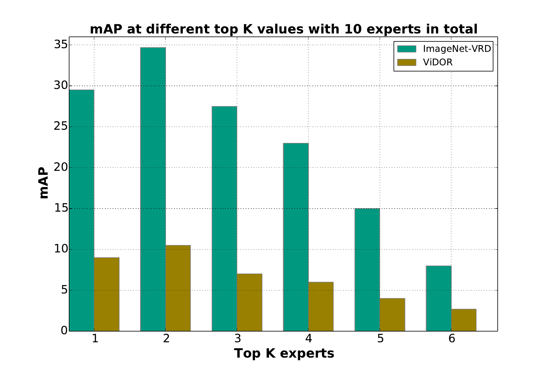
Multi-expert Performance
Our proposed MoE-VRD with \(K = 2\) and a total of \(N = 10\) experts,experts significantly outperforms state-of-the-art approaches on the ImageNet-VidVRD dataset across all evaluation criteria. The substantial performance boost is directly attributed to the mixture-of-experts strategy. Notably, the performance of our individual expert is comparable to the VidVRD-II method, as demonstrated in Table 1. The symbol "−" indicates that no corresponding results were reported for those entries.