Project Description
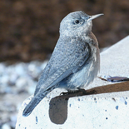
SLOPE_KP: Self-supervised Learning of Object Pose Estimation Using Keypoint Prediction presents a framework for estimating both object pose (camera perspective) and shape from a single image. The core contribution lies in leveraging self-supervised learning to detect semantically meaningful keypoints—characteristic locations on deformable objects (e.g., birds, cars)—without requiring manual annotations. By modeling these keypoints across an object category, SLOPE_KP enables accurate pose estimation while maintaining generalization across shape variations.
Key Contributions
- Co-managed the project in collaboration with research partners, overseeing stages from design and implementation to experimental evaluation and results dissemination.
- Designed and implemented a self-supervised pipeline for keypoint-based camera pose prediction and category-specific 3D shape reconstruction from single images.
- Developed experimental protocol using both static (CUB) and dynamic (YouTubeVos, DAVIS) datasets to evaluate model generalization across image and video domains.
- Executed large-scale training and testing of the model on high-performance computing clusters, handling diverse and high-volume visual data.
- Improved Mean-IoU by 8% and reduced 3D-Angular-Error of the pose by 5° for the CUB dataset.
Tools & Technologies
- Python, PyTorch, TensorFlow, Pandas, NumPy, Torchvision
- SoftRas, Neural Renderer, PyMesh
- OpenCV, scikit-learn, PIL (Pillow)
- Matplotlib (mpl_toolkits), Seaborn, Plotly, Visdom
- Container (Singularity, Docker)
- Cluster Computing, Parallel Computation
- Virtual Environment, Bash Environment
- Swedish National Infrastructure for Computing (SNIC)
Code / Git
Research / Paper
Additional Context
3D Geometry Fundamentals
In this section, I will explain the fundamentals of 3D geometry and rendering to provide a clearer understanding of the project and the proposed model.
Category-specific Mean Shape
The model's shape serves as a prototypical representation of a category, such as a bird, capturing the essential geometric structure common to that category. This allows the model to generalize across different instances while maintaining the key features that define the category. We have acces to the shape components of the category specific mean shape including Vertices, Faces, UV Vertices, and UV Faces.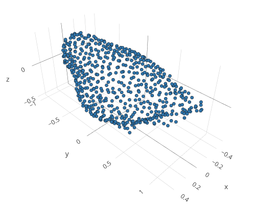
Shape
The shape of an object is defined by two fundamental components: vertices and faces.Vertices
Vertices represent the 3D points scattered across the surface of the object. These points define the structure and are arranged in a matrix of size \((V, 3)\), where \(V\) is the number of vertices, and each vertex contains three coordinates \((x, y, z)\) representing its position in 3D space.Faces
Faces are typically triangular surfaces formed by connecting three vertices. These triangles collectively form the surface of the object's 3D shape. The faces are organized in a structure of shape \((F, 3)\), where \(F\) represents the number of faces, and each face consists of three vertices.UV Vertices
This is an array containing UV coordinates for each vertex in the 3D model. It usually has the shape \((V, 2)\), where \(V\) is the number of vertices. Each entry contains the UV coordinates \((u, v)\) for a vertex.UV Faces
This is an array that specifies the texture coordinates (UV coordinates) for each face of the 3D model. It defines how the UV coordinates are connected to form faces in the texture space. It has shape of \((F, 3)\) where \(F\) is the number of faces and each entry contains three indices. These indices correspond to vertices in the UV Vertices array, forming triangles or other polygons in the 2D texture space.Texture
Texture refers to the detailed surface information that is applied to a 3D mesh. The texture is essentially a 2D image that gets mapped onto the 3D model to provide visual detail such as colors and patterns.
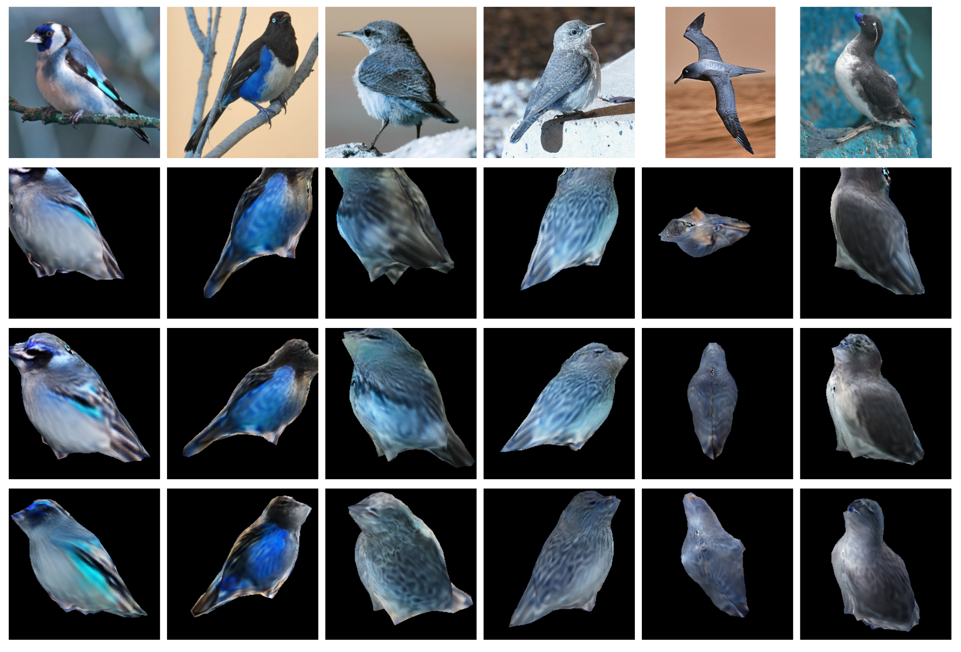
Texture Predictor
First The model’s TextureMapPredictor module outputs the predicted texture map. The texture map is essentially a 2D image (or multiple images) that captures the texture details to be applied to the 3D model. The shape of the texture map is \((B, C, H, W)\), where \(B\) is the batch size, \(C\) is the number of color channels (typically 3 for RGB or 2 if predicting flow), and \(H\) and \(W\) are the height and width of the texture image, respectively. The \(H\) and \(W\) dimensions correspond to the \(u\) and \(v\) coordinates in the texture/pixel space. We need a way to map the 2D texture map (image) onto the 3D surface of the model.
UV Sampler
Each face of the 3D model is associated with a set of UV coordinates (pixel coordinates of the 2D image) that specify how the texture (image pixels) should be wrapped around the model. The UV Sampler uses these coordinates to determine which parts of the texture (image) correspond to which parts of the 3D surface. The UV Sampler tensor has shape \((F, T, T, 2)\), where \(F\) is the number of faces, \(T\) is the texture size, and 2 is the \((u, v)\) coordinate. Each face has a texture with \((T \times T)\) pixels, and each pixel has a \((u,v)\) coordinate. By sampling these coordinates, the model can fetch the correct color or texture information from the 2D texture map. This process allows the model to apply detailed texture information to the 3D surface.
Sampling Results
The result of this sampling is a texture map for each face of the 3D model, which is then used to render or visualize the model. The sampled texture values correspond to the areas of the texture image that should appear on the model’s surface. After sampling, the texture has shape of \((B, F, T, T, C)\) indicating that for each face \(F\) in the 3D model, we get a \((T \times T)\) texture grid, with \(C\) channels of color (3) or flow (2) information.
Training Texture Prediction Model
Backpropagation involves updating the Texture Predictor Model, as it is responsible for generating the initial texture map from the input features. The loss is backpropagated to this model, allowing its parameters to be adjusted based on the gradients derived from the loss, thereby enhancing texture prediction accuracy. In contrast, the UV Sampler, which maps 2D texture coordinates to the 3D shape, is crucial for the final rendering but is typically a fixed function or non-learnable component. It does not have parameters that can be optimized, so the loss is not backpropagated to it.
Rendering
After obtaining the texture map outputs from the Texture Prediction Model, combined with the UV Sampling module, the resulting texture has the shape \((B, F, T, T, C)\). Along with the predicted vertices reconstructed from the deformations of the mean shape, as predicted by the Shape Model, we now have the 3D geometry and corresponding texture of the object necessary for rendering its image.
However, while the network predicts both the 3D shape and texture, the camera pose remains critical for accurately projecting this 3D data into a 2D image. Without the camera pose, it would be impossible to correctly position, orient, and map the texture of the 3D object onto the 2D image plane from the desired viewpoint. Our rendering function, therefore, takes as input the vertices, faces, 3D texture, and camera pose to generate the final rendered texture and mask.
3D Rotation
Euler Angles
I start by a short introduction to rotation. 3D rotation can be shown by three angles:
- Azimuth
This is the angle of rotation around the vertical axis (often the z-axis in spherical coordinate systems). It represents the angle in the horizontal plane from a reference direction, typically describing the yaw (left and right) rotation. - Elevation
This is the angle of rotation around the horizontal axis (often the y-axis or the x-axis depending on convention). It represents the angle in the vertical plane, effectively changing the pitch (up and down) of the object. - Cyclo-Rotation
This represents a rotation around the remaining third axis (usually the x-axis in many conventions). This angle corresponds to roll (tilting) of the object.
Gimbal Lock Phenomenon
In normal situations, the three axes of rotation (pitch, yaw, and roll) are independent, meaning that adjusting one does not affect the others. However, if you rotate the object in such a way that two of these axes align (for example, rotating 90 degrees in pitch), you lose the ability to rotate around one of the original axes. This is what causes gimbal lock: the system becomes "locked" in a way that removes one degree of freedom, and the object can no longer be oriented in certain ways. For example, in an airplane, if you pitch the plane 90 degrees (nose pointing straight up), the yaw and roll axes are now aligned, meaning that trying to adjust yaw will result in roll instead, and vice versa.
Rotation Matrices and Orthogonality
Rotation matrices are indeed orthogonal matrices:Preservation of Length and Angles: Rotation, by definition, should preserve the magnitude (or length) of vectors and the angles between them. Orthogonal matrices have the property of preserving the dot product between vectors, which guarantees that the vector lengths and angles are unchanged. This is crucial for rotations, as they only change the direction of vectors, not their size or relative orientation.
Invertible: Rotation matrices are required to be invertible, so that rotating by an angle and then rotating by the opposite angle returns the vector to its original position. Orthogonal matrices satisfy the property \(Q^{-1}=Q^T)=\). This simplifies calculations, as it means that the transpose of the rotation matrix can be used to perform the inverse rotation.
Determinant: The determinant of a rotation matrix is always +1. While orthogonal matrices can have determinants of If the determinant is −1, the matrix represents a reflection rather than a rotation.
Orthogonal Matrix
Transpose Equals Inverse
An orthogonal matrix \( Q \) satisfies the condition:
$$ Q^T Q = Q Q^T = I $$
where \( Q^T \) is the transpose of \( Q \) and \( I \) is the identity matrix. This means that the inverse of \( Q \) is its transpose: \( Q^{-1} = Q^T \).
Preserves Lengths and Angles
Multiplying a vector by an orthogonal matrix preserves the vector's length and the angle between vectors. This makes orthogonal matrices useful for transformations that involve rotations and reflections in geometry.
Determinant
The determinant of an orthogonal matrix is always \( +1 \) or \( -1 \). If the determinant is \( +1 \), the matrix represents a rotation. If it’s \( -1 \), it represents a reflection.
Orthonormal Rows and Columns
- Each row and each column of an orthogonal matrix is a unit vector.
- The rows (and similarly the columns) are orthogonal to each other.
Quaternions
Quaternions Goel et al. (2020) are a mathematical system that extends complex numbers, and they are often used in 3D graphics and physics to represent rotations in 3D space without suffering from issues like gimbal lock, which can occur with Euler angles (like azimuth, elevation, and cyclo-rotation). Quaternions provide a solution to gimbal lock because they represent rotations in 3D space without relying on three sequential angles. Instead of using Euler angles or a gimbal system, quaternions encode rotation as a single, continuous transformation in 3D space. This avoids the problem of gimbal lock entirely and provides smoother and more stable rotations A quaternion \(q\) has the form:
$$ q = w + xi + yj + zk = (w, \vec{v}) = (w, x, y, z)$$
where:- \(w\) is the scalar (real part).
- The scalar part \(w\) is related to the angle of rotation \(\theta\).
- \(x,y,z\) are the vector (imaginary) components.
- \(i,j,k\) are the fundamental quaternion units.
- The vector part \(x, y, z\) defines the axis of rotation. This is the direction in 3D space around which the rotation occurs.
$$ w = \cos\left(\frac{\theta}{2}\right), \; x = \sin\left(\frac{\theta}{2}\right) v_x, \; y = \sin\left(\frac{\theta}{2}\right) v_y, \; z = \sin\left(\frac{\theta}{2}\right) v_z $$
where \((v_x, v_y, v_z)\) is the unit vector of the axis of rotation, and \(\theta\) is the rotation angle in radians.Converting Euler Angles to Quaternions
Quaternions for Each Rotation are computed as following:
- Azimuth (Rotation around the z-axis)
\( q_{az} = \left( \cos\left(\frac{az}{2}\right), 0, 0, \sin\left(\frac{az}{2}\right) \right) \)
- Elevation (Rotation around the x-axis)
\( q_{el} = \left( \cos\left(\frac{el}{2}\right), \sin\left(\frac{el}{2}\right), 0, 0 \right) \)
- Cyclo-rotation (Rotation around the y-axis)
\( q_{rot} = \left( \cos\left(\frac{rot}{2}\right), 0, \sin\left(\frac{rot}{2}\right), 0 \right) \)
- Combining Quaternions
The combined quaternion \( q \) is obtained by multiplying these quaternions in the order of the rotation sequence. Assuming the order of rotations is azimuth (z-axis), elevation (x-axis), and cyclo-rotation (y-axis):
\( q = q_{rot} \times (q_{el} \times q_{az}) \)
where \( \times \) denotes quaternion multiplication (Hamilton product).
Gram-Schmidt
The 6D rotation representation mapped onto SO(3) using the partial Gram-Schmidt procedure Zhou et al. (2020) is a method to represent 3D rotations more efficiently and robustly than traditional methods like Euler angles or quaternions. Unlike Euler angles, the 6D representation avoids gimbal lock and discontinuities. Moreover, the representation is more numerically stable compared to quaternions, especially when used in optimization tasks (e.g., neural networks), since quaternions require normalization to maintain valid rotations.- 6D Representation
Instead of using 3 parameters (Euler angles) or 4 (quaternions) to represent a 3D rotation, this method uses a 6D vector. This 6D vector is derived from two orthogonal 3D vectors. These two vectors are then used to construct a rotation matrix. - Gram-Schmidt Procedure
The Gram-Schmidt process is a method for orthogonalizing a set of vectors. In this case, you begin with the two 3D vectors that form the 6D representation. Using Gram-Schmidt, these two vectors are orthogonalized to form the first two columns of a \(3 \times 3\) rotation matrix. The partial Gram-Schmidt process here focuses on constructing an orthogonal matrix that maps to SO(3) the space of 3D rotations.- The first vector becomes the first column of the rotation matrix.
- The second vector is orthogonalized relative to the first using the Gram-Schmidt procedure, forming the second column of the matrix.
- The third column is computed as the cross product of the first two columns to ensure that the resulting matrix lies in SO(3), i.e., it is a valid rotation matrix.
Special Orthogonalization Using SVD
The "special orthogonalization using SVD" Levinson et al. (2020) based on a 9D rotation representation, involves mapping a 9-dimensional (9D) vector to the special orthogonal group SO(3), which consists of valid 3D rotation matrices. This process leverages Singular Value Decomposition (SVD) to ensure the resulting matrix is a valid rotation matrix (i.e., it has orthonormal columns and a determinant of 1). The use of SVD ensures that the resulting matrix is orthogonal, which is a requirement for a valid rotation matrix. SVD is a well-established and stable algorithm, making this method robust for tasks that require precise rotation computations. This approach is flexible, and can handle matrices that are initially non-orthogonal, correcting them via the SVD process to ensure they represent a valid rotation.
- 9D Representation
The 9D rotation representation consists of a 9D vector reshaped into a \(3 \times 3\) matrix. This matrix may not initially satisfy the constraints required for a valid rotation matrix (i.e., orthogonality and determinant of 1). - Special Orthogonalization Using SVD
SVD (Singular Value Decomposition) is a factorization technique that decomposes a matrix \(\text{M}\) into three matrices:\( \text{M} = \text{U} \sum \text{V} \)
where:- \(\text{U}\) and \(\text{V}\) are orthogonal matrices,
- \(\sum\) is a diagonal matrix containing the singular values (which represent the scaling along each dimension).
\( \text{R} = \text{U} \text{V}^{\text{T}} \)
This ensures that \(\text{R}\) is a valid orthogonal matrix.
Additionally, to guarantee that \(\text{R}\) lies in SO(3) (i.e., that its determinant is +1), an adjustment is made if necessary:
If \(det(\text{R}) = -1\), the sign of one of the columns of \(\text{U}\) is flipped to ensure that \(\text{R}\) has a determinant of +1, making it a proper rotation matrix.
Model Architecture
- Shape Predictor
- Texture Predictor
- Camera-pose Predictor
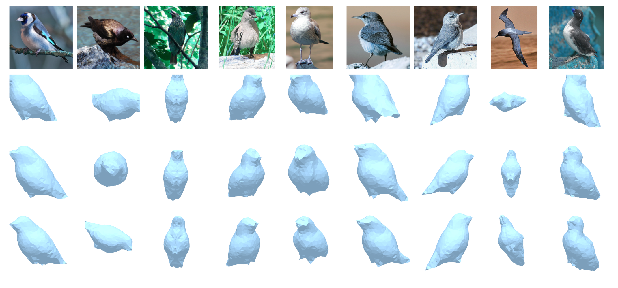
Shape prediction module is composed of N blocks of Convolutional Layers which receives image as input and outputs a tensor of size \(n_{\text{vertices}}\times 3\) representing deformation from a category-specific mean shape.
Texture prediction moduler reconstructs the RGB texture image of the 3D mesh. It applies a texture map predictor network to generate texture maps based on feature maps, and outputs an RGB texture image with dimensions of (\(\text{B}, \text{C}, \text{H}, \text{W}\)). After using UV Sampling to ensure accurate texture application, we obtain texture map with shape (\({B}, {F}, {T}, {T}, {C}\)), indicating that for each face \(F\) in the 3D model, we get a \((T \times T)\) texture grid, with \(C\) channels of color (3) or flow (2) information.
The pose is represented using an orthographic camera, parameterized by scale, translation, and rotation. Specifically, one parameter is used for scale, two for translation, and four for rotation, with unit quaternions representing the latter. Instead of directly predicting these parameters, we predict a set of keypoints that correspond to positions on the 3D category-specific mean shape. With these keypoint correspondences, a camera pose optimization algorithm, such as RANSAC Fisher et al. (1981), can be applied to determine the camera pose, as described below.
Phase-I: Camera Multiplex
We begin by optimizing a randomly initialized camera multiplex, which represents a distribution over 40 cameras. Each camera is initialized with 6 parameters: 1 for scale, 2 for translation, and 3 for Euler angle rotations representing Azimuth, Elevation and Cyclo-rotation. The goal is to find the camera configuration that best explains the image, considering varying object poses. During this process, the multiplex is pruned down to the 4 best cameras by minimizing a camera update loss, which is computed from the rendered masks and textures (reconstructed image).
Phase-II: Shape and Texture Reconstruction
In the next phase, using the pruned multiplex of the 4 best cameras, we train the shape and texture models. The camera multiplex continues to be optimized based on the camera update loss, calculated from the rendered masks, and texture (reconstructed image) until we converge on the single best camera configuration that captures the object's pose most accurately.The total loss to train shape and texture is defined as following:
\( L_{\text{total}} = \sum_{k} p_{k} \left(L_{\text{mask}, k} + L_{\text{pixel}, k}\right) + L_{\text{def}} + L_{\text{lap}}, \)
Where \(k\) indexes the cameras in the multiplex, and the silhouette mask loss is defined as:
\(L_{\text{mask}, k} = ||S - \tilde{S}_k||_2^2 + \text{dt}(S) \cdot \tilde{S}_k\)
where \(S\) and \(\tilde{S}_{k}\) are the ground-truth mask and the mask rendered from camera \(k\), respectively. \(dt(S)\) is the unidirectional distance transform of the ground-truth mask.
Unidirectional distance transform of the ground-truth mask: A distance transform converts a binary mask into a distance map, where each pixel's value represents the minimum distance to the nearest boundary or differently valued pixel (e.g., from foreground to background).Typically, distance transforms are calculated bidirectionally, measuring distances across both foreground-to-background and background-to-foreground transitions. In contrast, a unidirectional distance transform measures distance in only one direction—either from the foreground to the background or vice versa. For example, a unidirectional transform focused on foreground-to-background would measure how far each foreground pixel is from its nearest background pixel.
The image reconstruction loss computed from the foreground image is:
\(L_{\text{pixel}, k} = \text{dist}(\tilde{I}_k \odot S, I \odot S)\),
where \(I\) and \(\tilde{I}_k\) are the RGB image and the image rendered from camera \(k\). The \( \odot\) denotes the element-wise product.A graph-laplacian smoothness prior on the shape that penalizes the vertices \(i\) that are far away from the centroid of their neighboring vertices \(N(i)\):
\(L_{\text{lap}} = ||V_i - \frac{1}{|N(i)|} \sum_{j \in N(i)} V_j ||^2\),
For deformable objects like birds, it is beneficial to regularize the deformations to avoid arbitrary large deformations from the mean shape by adding the energy term:
\(L_{\text{def}} = ||\Delta {V}||\).
The probability that a camera \(k\) is the optimal choice is computed using:
\( p_{k} = \frac{e^{-\frac{L_k}{\sigma}}}{\sum_{j} e^{-\frac{L_j}{\sigma}}}, \)
where \(L_{k} = L_{\text{mask}, k} + L_{\text{pixel}, k}\) is the camera update loss.
Phase-III: Keypoint Pose Prediction
Finally using the best camera pose optimized by multiplex and trained shape and texture model, the camera pose is predicted.
Solving perspective-n-points by keypoint heatmaps
If object shapes are predicted as variations of a fixed model shape (mean shape) that has a set number of vertices and faces, then each object instance will have vertices that match the same semantic locations on the model. The only difference is their position due to deformation. These vertices can be treated as 3D keypoints. By reducing the number of keypoints through down-sampling and learning them from 2D images, we can use traditional methods, like robust PnP (Perspective-n-Point) estimators Campbell et al. (2020) to determine the object’s pose.
First, the object's shape is predicted as a deformation from a mean-shape or model shape, resulting in a new shape represented by 3D points. Next, \(N\) keypoints are randomly and uniformly selected from these 3D points using Farthest Point Sampling Qi et al. (2017). Using the best pose from the optimized the camera multiplex, these \(N\) keypoints are projected onto the image plane, resulting in corresponding 2D points. Finally, with these 3D and 2D points, we can solve the perspective-n-point (PnP) problem to estimate the camera's position and orientation relative to the scene.
Keypoints Prediction Loss
\( \theta = \text{arg min}_{\theta} \sum_{i}^{N} S_{w} || S_{h} - F(x_{i}; \theta) ||^2 \),
where a weighted least square loss function summed over all \(N\) keypoints applying the proxy ground-truth heatmaps \(S_h\) and the predicted heatmaps by \(F(x_{i}; \theta)\), which is a keypoint prediction network.
Keypoints Prediction Network \(F(x_{i}; \theta)\)
The keypoint prediction network consists of two components: the Smooth network and the Border network. The Smooth network includes a channel attention block, which selects discriminative features, and a refinement residual block to enhance the feature map at each stage of the feature extraction process. The Border network amplifies the distinction of features by using a semantic boundary to guide feature learning. To further increase inter-class distinction, the Border network explicitly learns the semantic boundary with supervised guidance.
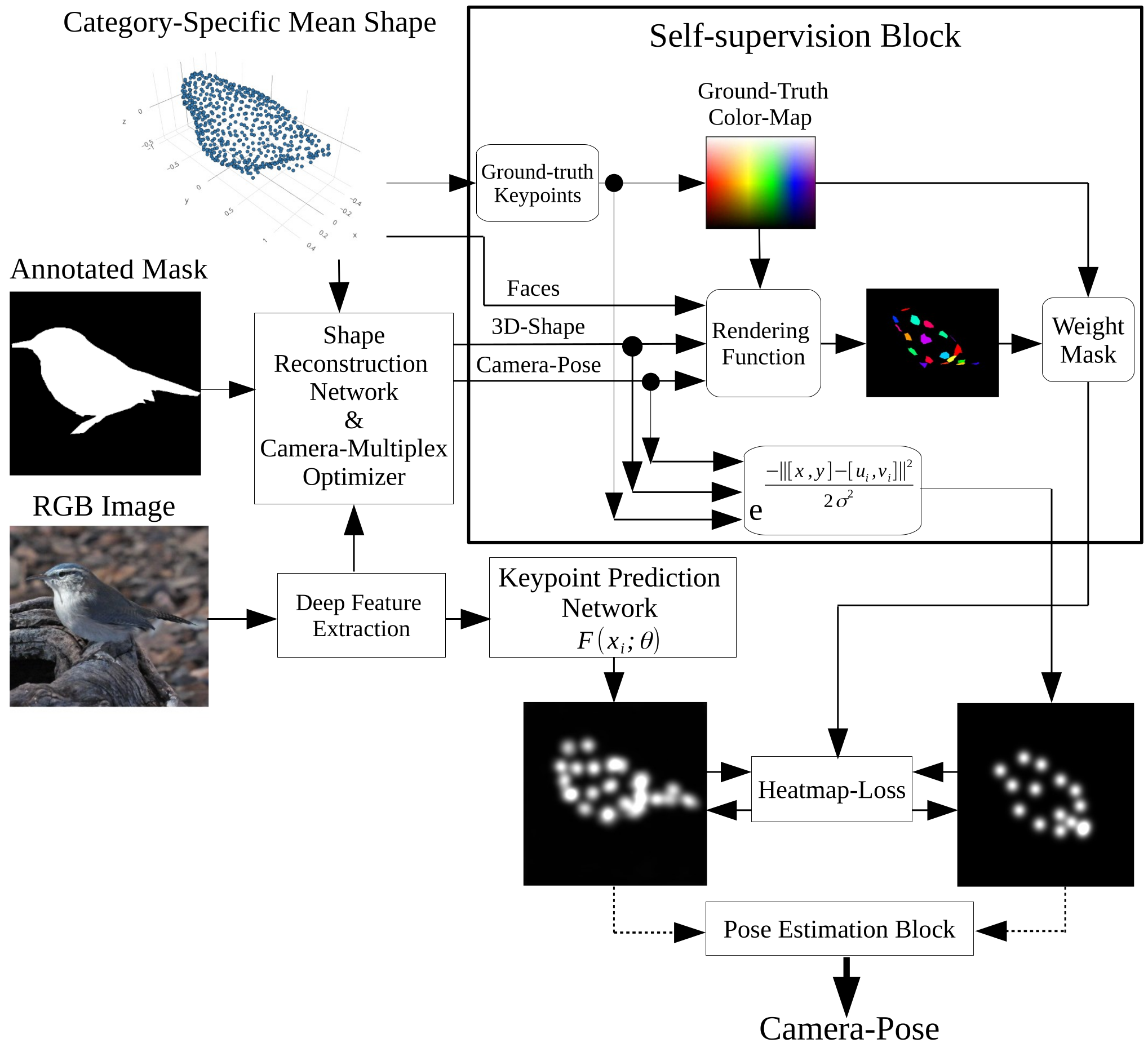
Self-supervision Block
The self-supervision block is developed to train the keypoints prediction network. This module is composed of two functional components \(S_h\) and \(S_w\) to generate a proxy ground-truth heatmaps and a weighting mask, respectively.
Rendered Label Texture (\(T_l\))
Due to the limitations in the used version of our renderer, a ground-truth label texture \(T_{\text{gt}}\) is initialized in the local coordinate space of the 3D model. The ground-truth texture data (colors) are created, without considering any external viewpoints (camera pose). To achieve this, a \(C_{\text{map}}\) assigns a unique color to each keypoint. Faces that contain at least one keypoint vertex are then colored according to.
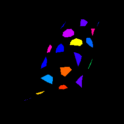
The rendering function projects the ground-truth label_texture \(T_{\text{gt}}\) onto the 3D model from the camera's viewpoint. It applies predicted vertices \(V\) representing the 3D coordinates of the model’s vertices, faces \(F\), which define the connectivity of these vertices to form the model's surface, and camera (best pose of multiplex \(\hat {\pi})\), which specifies the viewpoint and projection parameters. When \(T_{\text{gt}}\) is rendered using this function, it is mapped onto the model according to the camera’s perspective. The resulting output is a rendered texture \(T_{l}\) that visually integrates the color data from \(T_{\text{gt}}\) with the model’s geometry, as observed through the camera:
\( T_{l} = R (T_{\text{gt}}, F, V, \hat {\pi}) \),
Proxy Ground-truth Heatmaps (\(S_h\))
After the completion of Phase-II, we have an optimized multiplex, which gives of the best camera pose, as well as a trained shape reconstruction model, which predicts shape deformation \(\Delta V\), and texture. Applying random sampling of the 3D keypoints vertices over the object's predicted shape and best camera pose reconstructed by scale \(s\), translation \(t_{xy}\), and rotation \(r_q\), the 3D keypoints are projected into their 2D correspondences \([u_i, v_i]\). We employed \([x, y]\) as 2D coordinates of the image, and a Gaussian function to model the uncertainty of the locations of the 2D keypoints projections on the heatmap:
\( S_{h} = e^{\frac{-||[x, y] - [u_i, v_i] ||^2}{2 \sigma^2}} \).
Weighted Mask (\(S_w\))
The weight mask \(S_w\) is created by sampling colors \(c_{\text{sampled}}\) from the labeled texture \(T_{l}\), with each color corresponding to a 2D vertex \([u_i, v_i]\) that has been projected from a 3D keypoint.
\( S_{w} = \delta_{\epsilon}[||c_{\text{sampled}}-C_{\text{map}}||] \),
where \(\delta_{\epsilon}[arg]\) is an indicator, which returns 1 if its argument is true, and zero otherwise. The colors in \(C_{\text{map}}\) are chosen to be more than \(\epsilon\) apart, so it always works.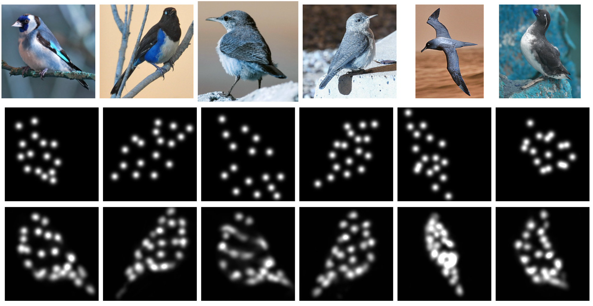
Experiments and Results
This section presents the experiment conducted with CUB Dataset Wah et al. (2011). We conducted our experiments to compare four different approaches to rotation representation. The first is to predict 4D unit quaternions by a CNN. The second is 6D rotation representation mapped onto SO(3) via a partial Gram-Schmidt procedure. The third is special orthogonalization using SVD based on 9D rotation representation. The fourth is our approach to camera pose prediction, which trains an intermediate keypoint prediction network.
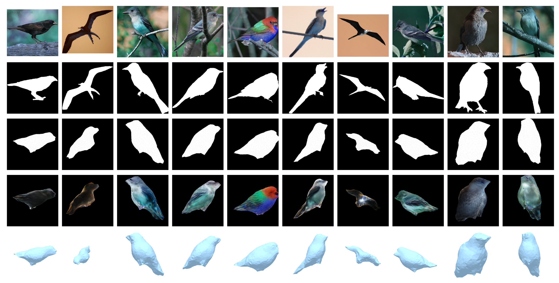
3D Mesh Reconstruction
Texture Reconstruction
Mask Reconstruction
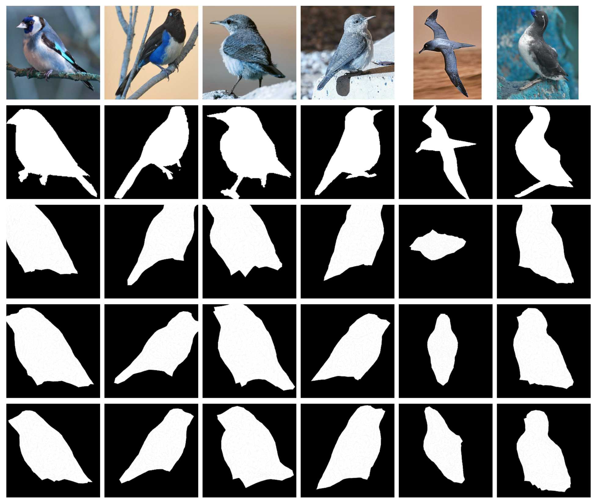
Image Reconstruction
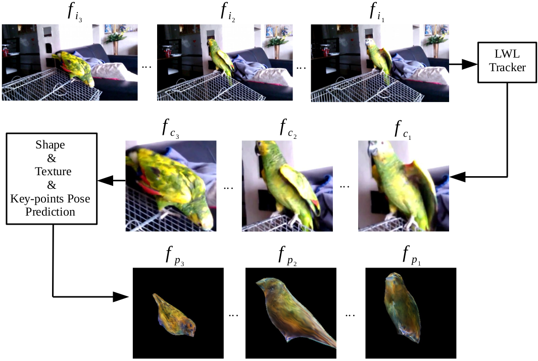
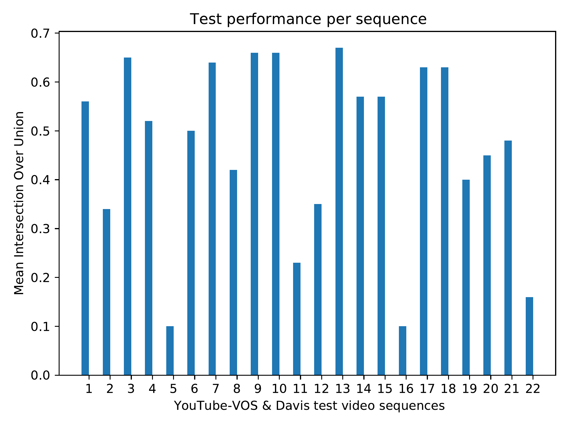
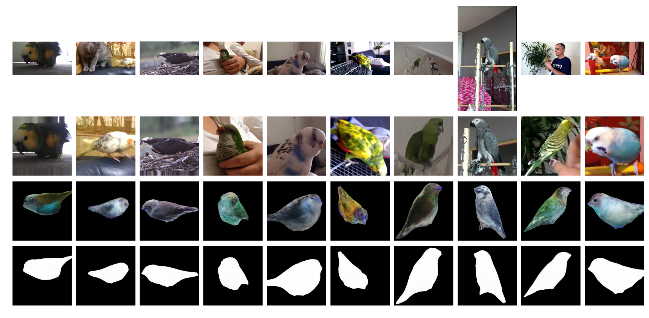
Online Inference 3D Object Reconstruction from Videos
We conduct online experiments to infer 3D objects from video sequences with single and multiple objects per image, using the YouTubeVos and Davis datasets Xu et al. (2018), and we focus on the bird category. Inferring objects from video sequences is challenging due to varying positions, orientations, and occlusions. We use LWL Bhat et al. (2020) to compute bounding boxes from the predicted masks. These bounding boxes are used to crop frames and create patches. The image patches are then input to the reconstruction network, which predicts shape, texture, and camera pose. We compare the masks reconstructed by our method and three other approaches against the ground-truth masks. Models are evaluated using three metrics: Jaccard-Mean (mean intersection over union), Jaccard-Recall (mean fraction of values exceeding a threshold), and Jaccard-Decay (performance loss over time).