Causal Implicit Models and Interventional Methods: ICRL-SM

Problem Motivation

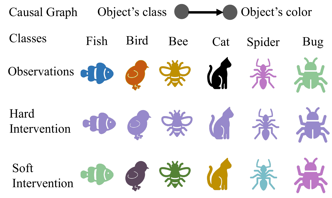
For instance, administering a drug can help determine whether a physiological effect is directly caused by a target factor or influenced by confounding variables. Assume a simplified setting in which exercise is the causal factor and heart rate is the observed physiological effect. Hard and soft interventions, such as a beta-blocker or external factors like caffeine, illustrate how interventions can modify observed outcomes and reveal underlying causal relationships. Accurately capturing these interventions is essential for models to reason reliably about mechanisms in biomedical and experimental settings.

(a) Cause-Effect observation: heart rate naturally increases with exercise in a controlled population.

(b) Hard intervention: A beta-blocker suppresses heart rate completely under controlled conditions (no caffeine, chocolate, or other stimulants), effectively breaking the causal effect of exercise.

(c) Soft intervention: A beta-blocker is applied in a non-controlled environment where participants may consume caffeine or other stimulants. Heart rate variation is partially restored, while the effect of exercise is still reduced compared to the no-intervention scenario.

Real-World Application

Soft interventions are especially relevant in vision, language, healthcare, and behavioral sciences. Real-world data often reflects subtle distributional shifts rather than clean experimental manipulations. This motivates models such as ICRL-SM, which are designed to learn robust causal representations under soft and ambiguous interventions.

Interventions

In causal modeling, an intervention refers to a deliberate manipulation of one or more variables to assess their causal influence on others within a system. By observing the outcomes of such manipulations, one can infer directional cause–effect relationships that go beyond statistical correlation. Interventions are typically categorized based on the level of control they exert over the causal system. Two fundamental types are Hard and Soft interventions.

Structural Causal Models (SCMs)

A Structural Causal Model (SCM) is defined as a tuple \( \mathcal{C} = (\mathcal{F}, \mathcal{Z}, \mathcal{E}, \mathcal{G}) \) with:

• A domain of causal variables \( \mathcal{Z} = \mathcal{Z}_1 \times \mathcal{Z}_2 \times \ldots \times \mathcal{Z}_n \)
• A domain of exogenous variables \( \mathcal{E} = \mathcal{E}_1 \times \mathcal{E}_2 \times \ldots \times \mathcal{E}_n \)
• A directed acyclic graph \( \mathcal{G}(\mathcal{C}) \) over causal and exogenous variables
• A set of causal mechanisms \( f_i \in \mathcal{F} \) mapping parent variables \( Z_{pa_i} \) and exogenous noise \( E_i \) to causal variable \( Z_i \)

Hard Interventions

Example: Suppose we are trying to understand the causal relationship between different types of diets and weight loss. If the government or an authority were to intervene and enforce a mandatory low-carb diet through legal means, this would constitute a hard intervention. In this scenario, regulations would be implemented, prohibiting the consumption of specific carbohydrate-containing foods. Regulatory agencies would be established to oversee and ensure adherence to the no-carb diet mandate, taking actions such as removing prohibited foods from the market, restricting their import and production, and so on. Individuals caught consuming banned foods would be subject to fines, legal repercussions, or other penalties.

Hard interventions forcibly set a variable to a fixed value, severing its dependence on any causal parents. This corresponds to the classical do-operator in SCMs. While theoretically powerful, such interventions are often impractical due to ethical, technical, or logistical constraints.

A hard intervention replaces the original causal mechanism of a variable \( Z \) with a constant value:

\( \tilde{z}_i = z^* \quad \text{(constant)}, \quad \text{independent of } z_{pa_i} \)

Graphically, this corresponds to deleting all incoming edges to the intervened node. A canonical example is a randomized controlled trial (RCT), where random assignment removes confounding by design.

Soft Interventions

Example: Suppose we are trying to understand the causal relationship between different types of diets and weight loss. The soft intervention in this scenario could be a switch from a regular diet to a low-carb diet. Switching to a low-carb diet is a voluntary choice made by the individual and there are no external forces or regulations compelling them to make this change (non-coercive). The intervention involves a modification of the individual’s diet rather than a complete disruption since they are adjusting the proportion of macronutrients (fats, proteins, and carbs) they consume. As a result, the causal variable (diet) is influenced by personal habits and other factors, so the intervention is subtle and does not completely break the causal influence of its parents.

Soft interventions modify the underlying causal mechanisms without fully overriding them. Rather than fixing a variable’s value, they perturb the functional or probabilistic relationships governing its behavior while preserving dependence on parent variables.

Formally, if a variable \( z_i \) is generated by \( f_i(z_{pa_i}, e_i) \) in the observational regime, a soft intervention modifies the conditional distribution:

\( p(z_i \mid z_{pa_i}) \rightarrow \tilde{p}(z_i \mid z_{pa_i}), \quad \tilde{z}_i = \tilde{f}_i(z_{pa_i}, \tilde{e}_i) \)

Unlike hard interventions, incoming edges to the intervened node remain intact, but the internal mechanism changes. This reflects real-world scenarios such as environmental shifts, policy changes, or behavioral nudges.

While more realistic, soft interventions introduce ambiguity: changes in observed variables may arise from either intervention or preserved parental influence, complicating causal discovery.

Causal Graph Structure

In many applications, the causal graph itself is unknown. While domain knowledge can sometimes specify the structure a priori, practical systems often require learning both the causal variables and their dependencies jointly. This has motivated two main approaches within the VAE framework: Explicit and Implicit Latent Causal Models.

Explicit Latent Causal Models (ELCMs)

ELCMs explicitly parameterize the adjacency matrix of a directed acyclic graph and enforce a factorized prior over latent variables:

\( p(z) = \prod_i p(z_i \mid z_{pa_i}) \)

This factorization improves interpretability, as each latent variable corresponds to a causal variable with explicit parent–child relationships. However, learning the graph structure and representations jointly often leads to unstable optimization and local minima.

Implicit Latent Causal Models (ILCMs)

Consider the following simple SCM:

\[ \begin{aligned} z_1 &= f_1(e_1) \\ z_2 &= f_2(z_1, e_2) \\ z_3 &= f_3(z_2, e_3) \end{aligned} \]

By recursively substituting upstream variables, each causal variable can be expressed purely in terms of exogenous noise:

\[ \begin{aligned} z_1 &= s_1(e_1) \\ z_2 &= s_2(e_2; e_1) \\ z_3 &= s_3(e_3; e_1, e_2) \end{aligned} \]

ILCMs avoid explicit graph learning by including all exogenous variables as inputs to solution functions. Relevant dependencies are learned implicitly, leading to more stable and scalable training. The trade-off is reduced structural interpretability.

Existing ILCMs primarily focus on hard interventions, limiting their applicability in real-world settings dominated by soft interventions. These subtle, non-deterministic shifts significantly complicate causal learning and motivate the approach taken in this project.

ICRL-SM: Implicit CRL via Switchable Mechanism

In the second problem we address implicit causal representation learning in the presence of soft intervention by using switch variable.

Problem formulation

Learning causal representations from observational and interventional data, especially when ground-truth structural causal graph (SCM) are unknown, is quite challenging. There are two main approaches to causal representation learning in the absence of ground-truth causal graph.

Implicit CRL via Interventions

Implicit causal representation learning (CRL) typically utilizes two types of interventional data: hard and soft interventions. In real-world scenarios, soft interventions are often more practical, as hard interventions require fully controlled environments. While the literature extensively studies implicit CRL with hard interventions, soft interventions offer a different approach by indirectly influencing the causal mechanisms rather than directly altering a causal variable. However, the nuanced nature of soft interventions poses additional challenges in accurately learning causal models.

Hard vs Soft Intervention

In a causal model, an intervention is a deliberate action to manipulate one or more variables to observe its impact on others, revealing causal relationships. Interventions can be categorized based on the level of control: hard and soft interventions.

hard intervention It directly sets the value of a causal variable, represented as \(do(Z = z)\), completely isolating the variable from the influence of its ancestral nodes.

soft intervention It indirectly modifies a variable by changing its conditional distribution, \(p(Z|Z_{pa}) \rightarrow \tilde{p}(Z|Z_{pa})\), allowing it to still be influenced by its parent nodes. This means the post-intervention value of \(\tilde Z\) is still influenced by its causal parents. As a result, the solution function \(\tilde s\) for the causal variable is affected by the intervention, making it harder to identify the causal mechanisms involved.

Switchable Mechanism

In hard intervention we are fully certain that changes in casual variables are direct result of intervention. While Soft interventions provide fewer constraints on the causal graph structure than hard interventions. This is because the connections to parental variables remain intact, leading to ambiguity in determining the causal relationships.

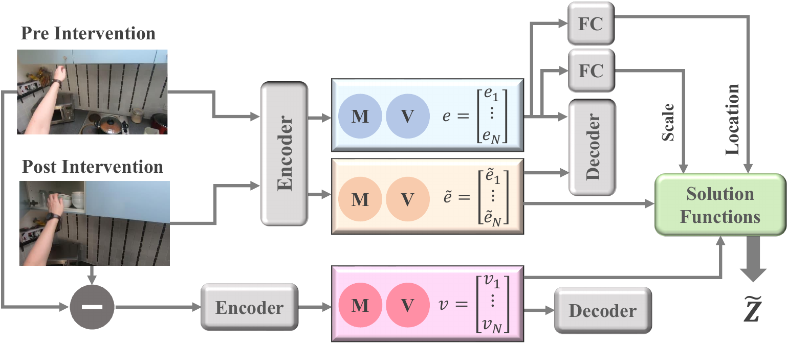
Data Augmentation

If our model include a data augmentation step that adds the intervention displacement \(\tilde x - x\) as an observed feature. This feature directly captures the full effect of the soft intervention in the observation space, making it easier to analyze its impact.

Application of Switch Variable

The switch variable allows the model to transition to the pre-intervention causal mechanisms when analyzing post-intervention data. In the post-intervention condition, our goal is to learn the representation of each causal variable \(p(\tilde z)\). While soft interventions maintain the ancestral connections to a causal variable (implying we should learn \(p(\tilde z|e_{pa})\)), these connections remain unknown due to the implicit nature of our learning method. To address this challenge, we model the post-intervention causal variable using its only known parent, which is its own exogenous variable, represented as \(p(\tilde z|e_{pa})\). The switch variable helps isolate changes in the intrinsic characteristics of each causal variable, encapsulated within its own exogenous variable. This improves the model's ability to learn causal relationships accurately.

Modulated Form of \(V\)

A modulated version of V is used in each causal variable’s solution function. The nonlinear function \(h_i: V \rightarrow R\) allows the model to account for variations in the parental sets of all causal variables. The equation \(z_i = s_i(e_i; e_{/i}) = s_i(e_i; e_{/i}, h_i(v))\) illustrates how the switch variable \(V_i \in R\) is incorporated into the solution functions for each causal variable \(Z_i\).

Augmented Implicit Causal Model

The inclusion of switch variables in the solution functions leads to the concept of an augmented implicit causal model. This model is designed to enhance the learning of causal relationships, especially in the context of soft interventions.

A solution function using a location-scale noise models, which defines an invertible diffeomorphism is formulated as follows:

\( z_i = \tilde{s}_i(\tilde{e}_i; e_{/i}, h_i(v)) = \frac{\tilde{e}_i - (\text{loc}_i(e_{/i}) + h_i(v))} {\text{scale}_i(e_{/i})} \)

Experiments