Causality Projects: GCRL & ICRL-SM

Overview

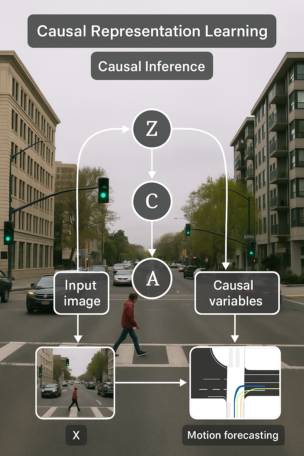
Here I will present two interesting projects with causality and causal representation learning; GCRL: Generative Causal Representation Learning for Out-of-Distribution Motion Forecasting, and ICRL-SM: Implicit Causal Representation Learning via Switchable Mechanism.

Causality

In this section, I will explain the fundamentals of causality and causal models required to better understand the ideas of these projects.

Structural Causal Models (SCMs)

Structural Causal Models (SCMs) are a way of describing causal features and their interactions, which are represented by Directed Acyclic Graphs (DAG) (Pearl et al., 2016).

We say that X is a direct cause of Y when there is a directed edge from X to Y in the DAG. The cause and effect relation X → Y tells us that changing the value of X can result in a change in the value of Y, but that the reverse is not true.

A causal model receives as inputs:

• A set of qualitative causal assumptions (A)
• A set of queries concerning the causal relations among variables (Q)
• Experimental or non-experimental data (D), presumably consistent with (A).

A causal model makes predictions about the behavior of a system. The outputs of a causal model are:

• A set of logical implications of (A)
• Data-dependent claims (C) represented by the magnitude or likelihoods of the queries (Q)
• A list of testable statistical implications (T).

Causal Variables

In causal analysis, variables are categorized into endogenous and exogenous variables, each playing distinct roles in understanding causal relationships.

• Endogenous Variables:

  Endogenous variables are influenced by other variables within the system. Their values are determined by interdependencies and causal relationships within the model. For example, in an economic model, consumer spending (Y) is an endogenous variable influenced by income (X), where an increase in income generally leads to an increase in spending.

• Exogenous Variables:

  Exogenous variables are determined outside the system being studied and do not depend on other variables in the model. They serve as external inputs that can affect endogenous variables. For instance, in the same economic model, factors like government policy changes or interest rates (X) can influence income but are not affected by consumer spending.

Causal Representation Learning (CRL)

Causal Representation Learning (CRL) is an emerging field within machine learning and artificial intelligence that focuses on learning representations of data that explicitly capture the underlying causal structures and relationships among variables. The goal is to improve understanding and predictions of complex systems by leveraging causal knowledge rather than solely relying on correlations.

• Causality vs. Correlation:

  Traditional machine learning often relies on correlations between variables, which can lead to misleading conclusions. For example, two variables may be correlated without one causing the other. CRL aims to identify causal relationships, helping to distinguish true causes from mere associations.

• Structural Causal Models (SCMs):

  SCMs are a mathematical framework used in CRL to represent causal relationships through Directed Acyclic Graphs (DAGs). Each node in the graph represents a variable, and directed edges indicate causal influences. This graphical representation enables clear understanding of how changes in one variable can affect others.

• Causal Inference:

  CRL incorporates techniques from causal inference, which involves drawing conclusions about causal relationships from data. This often involves interventions (manipulating variables) and counterfactual reasoning (considering what would happen under different circumstances).

• Interventions and Do-Calculus:

  Interventions (denoted as do-operations) are essential for causal analysis. CRL seeks to learn representations that can effectively simulate the effects of interventions on various variables. Do-calculus provides a formal framework for reasoning about these interventions.

• Latent Variables:

  CRL often deals with latent variables—unobserved factors that influence observed data. By capturing these latent structures, CRL can provide richer, more nuanced representations that enhance the model's predictive power.

• Implicit vs. Explicit CRL:
  • Explicit Causal Representation Learning involves direct modeling of causal relationships using known structures, such as SCMs or DAGs. When the causal graph is known, we can specify relationships directly, enabling accurate causal inference and intervention simulation.
  • Implicit Causal Representation Learning refers to inferring causal relationships from data without a clearly defined causal graph. This approach often relies on statistical techniques and causal discovery algorithms to hypothesize causal structures from observed correlations. The challenge lies in identifying true causal relationships amidst potential spurious associations.

Confounders

• Role in Causal Inference: Confounders can obscure or exaggerate the true causal relationship between variables, making it challenging to accurately identify and quantify causal effects.
• Identification: To correctly infer causal relationships, it's crucial to identify and control for confounders in the analysis. This often involves statistical techniques or domain knowledge to account for these variables.
• Example: Suppose you are studying the effect of exercise on weight loss. If you don’t account for diet, which influences both exercise habits and weight loss, you might incorrectly attribute changes in weight solely to exercise when diet also plays a significant role. In this case, diet is a confounder.
• Adjustment: In causal graphs, confounders are usually represented and accounted for to ensure that the relationships between variables are accurately estimated. Techniques such as stratification, regression, or matching can be used to adjust for confounding effects.

Backdoor Criterion

The backdoor criterion is a fundamental concept in causal inference, particularly when using Structural Causal Models (SCMs) and Directed Acyclic Graphs (DAGs). It provides a method to identify a set of variables that, when controlled for, can help estimate the causal effect of one variable on another, effectively eliminating confounding.

• Definition:

  The backdoor criterion states that a set of variables Z satisfies the backdoor criterion relative to two variables X and Y if:

  • Z blocks all backdoor paths from X to Y (i.e., paths that go into X and then to Y).
  • Z does not include any descendant of X.

• Backdoor Paths:

  A backdoor path is a path that connects X to Y that goes backwards through other variables (i.e., it starts with X and then moves to a variable that leads back to Y). Backdoor paths can introduce confounding bias in estimating the causal effect from X to Y.

• Causal Effect Estimation:

  By controlling for the variables in Z that satisfy the backdoor criterion, you can estimate the causal effect of X on Y using the expression p(Y | do(X)), which represents the distribution of Y when X is intervened upon (i.e., manipulated directly rather than just observing it).

• Example:

  Consider the following variables in a DAG:

  • X: Treatment (e.g., a new medication)
  • Y: Outcome (e.g., health improvement)
  • Z: Confounding variables (e.g., age, pre-existing health conditions)
  If both Z and another variable S affect both X and Y, then Z satisfies the backdoor criterion because it can block the backdoor paths from X to Y. By controlling for Z, you can obtain a more accurate estimate of the causal effect of X on Y.

GCRL: Generative CRL for Out-of-Distribution Motion Forecasting

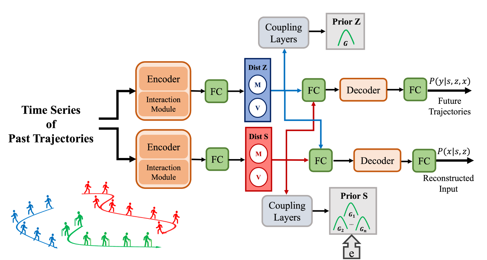
Causal formalism

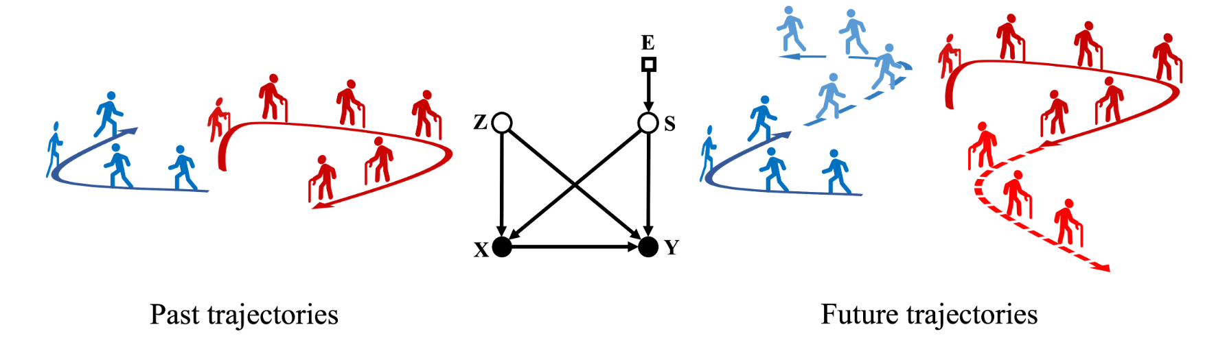
Figure (2) illustrates our proposed causal formalism for this project. Shown by figure (2) (center), we assume a known SCM, and two causal variables, which affect trajectories of the pedestrians:

• Invariant features do not vary across domains but can influence the trajectories of the pedestrians. These features can be associated with physical laws, traffic laws, social norms, and etc.
• Variant features vary across domains and can be associated with the motion styles of the pedestrians in an environment
.

Moreover, we consider four endogenous variables for different representations:

• S for variant features (unobserved/latent)
• Z for invariant features (unobserved/latent)
• X for past trajectories (observed)
• Y for future trajectories (observed)

We also introduce an additional exogenous variable shown by E as the selection variable to account for the changing factors in each environment. The selection variable acts as an identifier of an environment. In other words, we assume that all members of the dataset are sampled from a parent distribution over X, Y , and E.

Furthermore, we assume that the proposed model is causally sufficient where it explains all the dependencies without adding further causal variables.

Knowing the context of our causal model, the following conditions must be satisfied, which results in the edges formation of the causal graph:

• There should be an edge from S to X and Y because motion styles can influence the speed of the pedestrians.
• There should be an edge from Z to X and Y because social norms can influence how closely pedestrians move next to each other.
• There should be an edge from X to Y because the location in the past determines where the pedestrian is going to be in the future.
• S varies in each domain, hence, there should be an edge from selection variable E to S to account for all the changing factors in each domain.

Learning latent variables

Loss function

\( \text{loss} = \max_{p,q} \, \mathbb{E}_{p^*(x,y)} \left[ \log q(y|x) + \frac{1}{q(y|x)} \, \mathbb{E}_{q(s|x), q(z|x)} \left[p(y|x,s,z) \log\left(\frac{p(x|s,z) \, p(s) \, p(z)}{q(s|x) \, q(z|x)}\right)\right] \right] \)

where the loss is designed to address the following objectives if the optimal loss obtained:

1. To minimize the distance between ground-truth future trajectories Y and predicted future trajectories via maximizing the log likelihood posterior \(\log q(y|x)\).
2. To eliminate the confounding effect by estimating the causal effect of X on Y through \(\log q(y|x) = \mathbb{E}_{q(s|x), q(z|x)} p(y|x,s,z) = p(y|do(x)) \)
3. Reconstruction of the past trajectories X through maximizing \(\log(x|s,z)\)
4. Invariant representation learning through maximizing \(\log {\frac{p(z)}{q(z|x)}}\). Possible if q(z|x) = p(z) which means posterior equals prior.
5. Variant representation learning through maximizing \(\log {\frac{p(s)}{q(s|x)}}\). Possible if q(s|x) = p(s) which means posterior equals prior.

As discussed earlier latent variable S varies in each domain, so is domain-specific. Therefore, we model its prior with a Gaussian Mixture Model GMM, which are proven to be identifiable. Moreover, GMMs are universal approximators, hence, \(q(s|x)\) will be capable of producing arbitrary variant features

On the other hand latent variable Z is invariant and is the same in all domains, so we model its prior with a single Gaussian distribution.

Domain Adaptation

After the model is trained using our objective function, \(q(z|x)\) will generate representations with a single Gaussian distribution and \(q(s|x)\) will generate representations with a Gaussian Mixture Model (GMM) distribution. Therefore, all representations generated by \(q(z|x)\) will be in the same range, whereas the representations of \(q(s|x)\) will form clusters, each modeled by a component of the GMM.

What needs fine-tuning?

Since S can be interpreted as a weighted sum of the representations learnt from different environments of the training domains, which may be used in the test domains as well. Depending on how related the test domains are to the training domains, we may need to fine-tune the components of the S prior (GMM) to obtain a new prior for S. The models to predict future trajectories \(p(y|x, s, z)\) and to reconstruct past trajectories \(p(x|s, z)\) also needs to be fine-tuned as the samples of \(q(s|x)\) will be updated. Thus, we fine-tune \(p(y|x, s, z)\), \(p(x|s, z)\), \(q(s|x)\) and p(s).

What needs no fine-tuning?

Since Z is invariant, we can directly transfer it to the new domain without any fine-tuning. Thus \(p(z)\), and \(q(z|x)\) do not require fine-tuning, so they can be arbitrary complex.

How to conduct inference?

Experiments

1-Robustness

\(\gamma_t := (\dot{x}_{t+\delta t} - \dot{x}_t)^2 + (\dot{y}_{t+\delta t} - \dot{y}_t)^2\)

\(\sigma_t := \alpha(\gamma_t + 1)\)

where \(\dot{x}_t = x_{t+1} - x_t\) and \(\dot{y}_t = y_{t+1} - y_t\) reflect the velocity of the pedestrians within the temporal window length of \(\delta t = 8\), and \(\alpha\) is the noise intensity. For the training domains, \(\alpha \in \{1, 2, 4, 8\}\) while for the test domain, \(\alpha \in \{8, 16, 32, 64\}\). The test domain is the eth environment for this experiment. The results in Table 1 Gale Bagi et al., 2023. demonstrate the robustness of our method against observation noise while performing comparably with other motion forecasting models for low \(\alpha\).

2-Domain Generalization

To test domain generalization capabilities of GCRL, we consider the Minimum Separation Distances (MSD) in the training and test domains are \(\{0.1, 0.3, 0.5\}\) and \(\{0.1, 0.2, 0.3, 0.4, 0.5, 0.6, 0.7, 0.8\}\) meters, respectively. As illustrated in Figure 6 Gale Bagi et al., 2023, our method is more robust to domain shifts compared to baseline, and it is achieving slightly better ADE, which is 8.8% on average. For OOD-Inter cases, where the test domain shift falls within the range of training domain shifts (e.g., test domain shift = 0.4), GCRL remains reusable as ADE shows insensitivity to these shifts. However, for OOD-Extra cases, where test domain shifts lie outside the range of training domain shifts, the model requires fine-tuning to maintain performance.

3-Domain Adaptation

To evaluate the efficiency of our proposed method for knowledge transfer using a synthetic dataset under an OOD-Extra case. We train both baseline and GCRL with a consistent setup and fine-tune various model components using a limited number of batches from the test domain. Each batch contains 64 samples, resulting in fine-tuning with sample sizes of \(\{1, 2, 3, 4, 5, 6\} × 64\). For baseline, we fine-tune with the optimal settings reported in their paper. For GCRL, we fine-tune the components \( p(y|x, s, z) \), \( p(x|s, z) \), \( p(s) \), and \( q(s|x) \).

As illustrated in Figure 7 Gale Bagi et al., 2023, GCRL adapts to the new environment more rapidly and demonstrates greater robustness to OOD-Extra shifts compared to baseline, improving evaluation metric by an average of 34.3% over baseline.

4-Generative Bonus

Since GCRL is a generative approach, we can generate multiple future trajectories per sample and select the best of them to tackle the multi-modality of trajectories. Therefore, we use a hyper-parameter N in testing to determine the number of generated trajectories per sample. Figure 4 Gale Bagi et al., 2023 illustrates the significant impact that a generative approach can have in the performance. According to Figure 5 Gale Bagi et al., 2023 the qualitative results also suggest that a generative approach can be useful in motion forecasting as it is able to generate diverse trajectories.

ICRL-SM: Implicit CRL via Switchable Mechanism

In the second problem we address implicit causal representation learning in the presence of soft intervention by using switch variable.

Problem formulation

Learning causal representations from observational and interventional data, especially when ground-truth structural causal graph (SCM) are unknown, is quite challenging. There are two main approaches to causal representation learning in the absence of ground-truth causal graph.

Explicit CRL

Explicit Latent Causal Models (ELCMs) starts with an initial known causal graph structure reflecting our understanding of the relationships between variables, which is informed by domain knowledge, prior research, or theoretical considerations. This initial graph indicates potential causal relationships among variables, even if the exact strength and direction of these relationships remain unquantified. Accompanying this graph is an adjacency matrix that contains initial estimates of causal relationships, represented as zeros for no direct relationship or other values indicating the strength of influence.

During training, the model refines the parameters associated with the graph's edges using observed data to estimate coefficients that quantify the causal relationships. As the model learns, it adjusts the parameters in the adjacency matrix to improve its fit to the observed data while maintaining the specified structure.

The training process incorporates conditions to ensure identifiability, aiming to achieve an optimal graph structure that accurately identifies causal relationships from the data. Upon completion of training, the model may refine the initial graph structure based on the learned parameters, which can result in modifications to the edges or directions of causation.

Implicit CRL

In Implicit Latent Causal Models (ILCMs), the absence of a predefined causal graph means that the model does not start with explicit knowledge about how variables are related causally. Instead, the model relies on observed data to infer the underlying causal mechanisms. This process often involves statistical techniques and causal discovery algorithms that analyze correlations and dependencies within the data to hypothesize causal relationships.

The solution function learned during this process represents the causal representation of the variables involved. This function encapsulates the cause-and-effect relationships identified from the data, allowing for the prediction of outcomes based on interventions or changes in certain variables.

However, unlike explicit CRL, where the aim is to refine a causal graph and adjacency matrix, implicit CRL focuses on estimating the effects of interventions without explicitly modeling the causal structure. The primary challenge in implicit CRL is to ensure that the learned relationships are valid and robust against potential confounding factors or spurious associations present in the data. The goal is to identify true causal effects that can be reliably used for prediction and decision-making, even in the absence of a clear graphical representation of the underlying causal system.

Implicit CRL via Interventions

Implicit causal representation learning (CRL) typically utilizes two types of interventional data: hard and soft interventions. In real-world scenarios, soft interventions are often more practical, as hard interventions require fully controlled environments. While the literature extensively studies implicit CRL with hard interventions, soft interventions offer a different approach by indirectly influencing the causal mechanisms rather than directly altering a causal variable. However, the nuanced nature of soft interventions poses additional challenges in accurately learning causal models.

Hard vs Soft Intervention

In a causal model, an intervention is a deliberate action to manipulate one or more variables to observe its impact on others, revealing causal relationships. Interventions can be categorized based on the level of control: hard and soft interventions.

hard intervention It directly sets the value of a causal variable, represented as do(Z = z), completely isolating the variable from the influence of its ancestral nodes.

Example: Suppose we are trying to understand the causal relationship between different types of diets and weight loss. If the government or an authority were to intervene and enforce a mandatory low-carb diet through legal means, this would constitute a hard intervention. In this scenario, regulations would be implemented, prohibiting the consumption of specific carbohydrate-containing foods. Regulatory agencies would be established to oversee and ensure adherence to the low-carb diet mandate, taking actions such as removing prohibited foods from the market, restricting their import and production, and so on. Individuals caught consuming banned foods would be subject to fines, legal repercussions, or other penalties.

soft intervention It indirectly modifies a variable by changing its conditional distribution, \(p(Z|Z_{pa}) \rightarrow \tilde{p}(Z|Z_{pa})\), allowing it to still be influenced by its parent nodes. This means the post-intervention value of \(\tilde Z\) is still influenced by its causal parents. As a result, the solution function \(\tilde s\) for the causal variable is affected by the intervention, making it harder to identify the causal mechanisms involved.

Example: Suppose we are trying to understand the causal relationship between different types of diets and weight loss. The soft intervention in this scenario could be a switch from a regular diet to a low-carb diet. Switching to a low-carb diet is a voluntary choice made by the individual and there are no external forces or regulations compelling them to make this change (non-coercive). The intervention involves a modification of the individual’s diet rather than a complete disruption since they are adjusting the proportion of macronutrients (fats, proteins, and carbs) they consume, which is less disruptive than a radical change in eating habits (gradual modification).

Switchable Mechanism

In hard intervention we are fully certain that changes in casual variables are direct result of intervention. While Soft interventions provide fewer constraints on the causal graph structure than hard interventions. This is because the connections to parental variables remain intact, leading to ambiguity in determining the causal relationships.

Data Augmentation

If our model include a data augmentation step that adds the intervention displacement \(\tilde x - x\) as an observed feature. This feature directly captures the full effect of the soft intervention in the observation space, making it easier to analyze its impact.

Application of Switch Variable

The switch variable allows the model to transition to the pre-intervention causal mechanisms when analyzing post-intervention data. In the post-intervention condition, our goal is to learn the representation of each causal variable \(p(\tilde z)\). While soft interventions maintain the ancestral connections to a causal variable (implying we should learn \(p(\tilde z|e_{pa})\)), these connections remain unknown due to the implicit nature of our learning method. To address this challenge, we model the post-intervention causal variable using its only known parent, which is its own exogenous variable, represented as \(p(\tilde z|e_{pa})\). The switch variable helps isolate changes in the intrinsic characteristics of each causal variable, encapsulated within its own exogenous variable. This improves the model's ability to learn causal relationships accurately.

Modulated Form of V

A modulated version of V is used in each causal variable’s solution function. The nonlinear function \(h_i: V \rightarrow R\) allows the model to account for variations in the parental sets of all causal variables. The equation \(z_i = s_i(e_i; e_{/i}) = s_i(e_i; e_{/i}, h_i(v))\) illustrates how the switch variable \(V_i \in R\) is incorporated into the solution functions for each causal variable \(Z_i\).

Augmented Implicit Causal Model

The inclusion of switch variables in the solution functions leads to the concept of an augmented implicit causal model. This model is designed to enhance the learning of causal relationships, especially in the context of soft interventions.

A solution function using a location-scale noise models, which defines an invertible diffeomorphism is formulated as follows:

\( z_i = \tilde{s}_i(\tilde{e}_i; e_{/i}, h_i(v)) = \frac{\tilde{e}_i - (\text{loci}(e_{/i}) + h_i(v))} {\text{scale}_i(e_{/i})} \)

Experiments

Tools and Technologies

This section discusses the design and implementation of the project.

Data Visualization

Utilized various libraries for data visualization:

• Matplotlib
• Seaborn
• Plotly
• Visdom

Links

Overview of the links related to the projects:

Version Control Systems:

• GCRL GitHub Page

Research Article Platforms:

• GCRL Paper
• ICRL-SM Paper