Images
The BIOSCAN-5M dataset contains 5,150,808 high-quality images of living organisms.
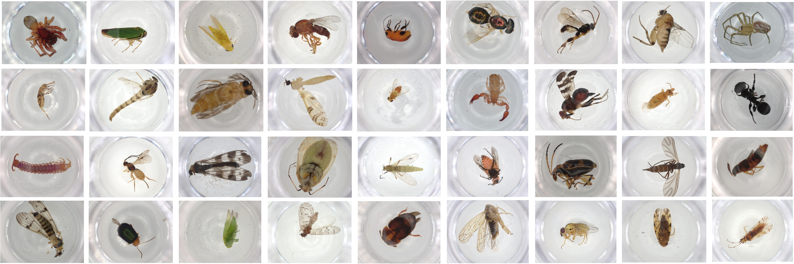
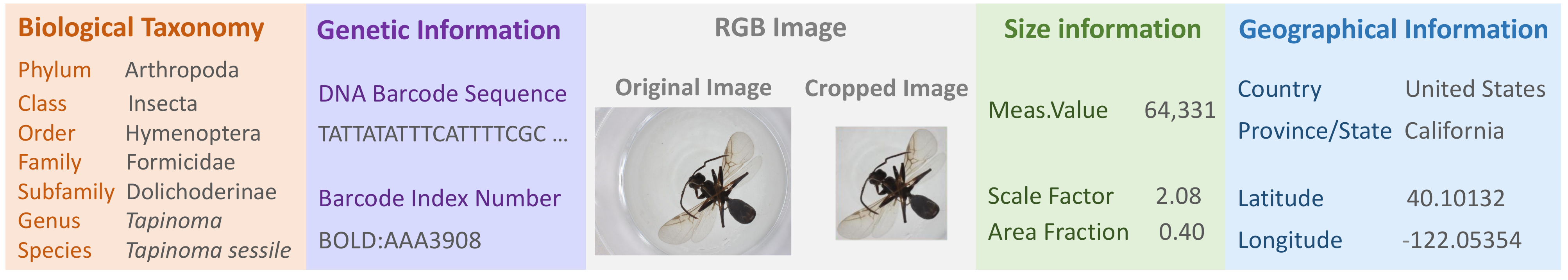
This project introduced a large-scale dataset of over five million samples, each consisting of a high-quality microscopic RGB image, a DNA barcode sequence, and a Barcode Index Number. The dataset comprises both structured and unstructured data formats. Structured data, provided in CSV and JSON-LD formats, includes taxonomy labels, DNA sequences, Barcode Index Numbers, geographic metadata, and specimen size information. Unstructured data consists primarily of images.
The BIOSCAN-5M dataset contains 5,150,808 high-quality images of living organisms.
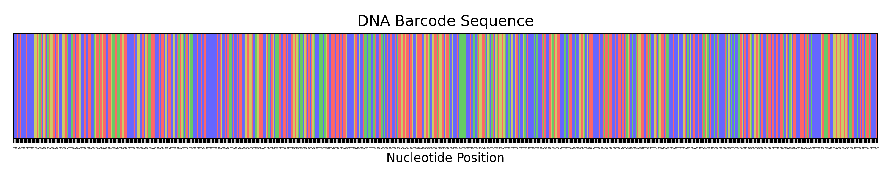
The presented DNA barcode sequence illustrates the nucleotide arrangement—Adenine (A), Thymine (T), Cytosine (C), and Guanine (G)—within a designated gene region, such as the mitochondrial cytochrome c oxidase subunit I (COI) gene.
TTTATATTTTATTTTTGGAGCATGATCAGGAATAGTTGGAACTTCAATAAGTTTATTAATTCGAACAGAATTAAG...
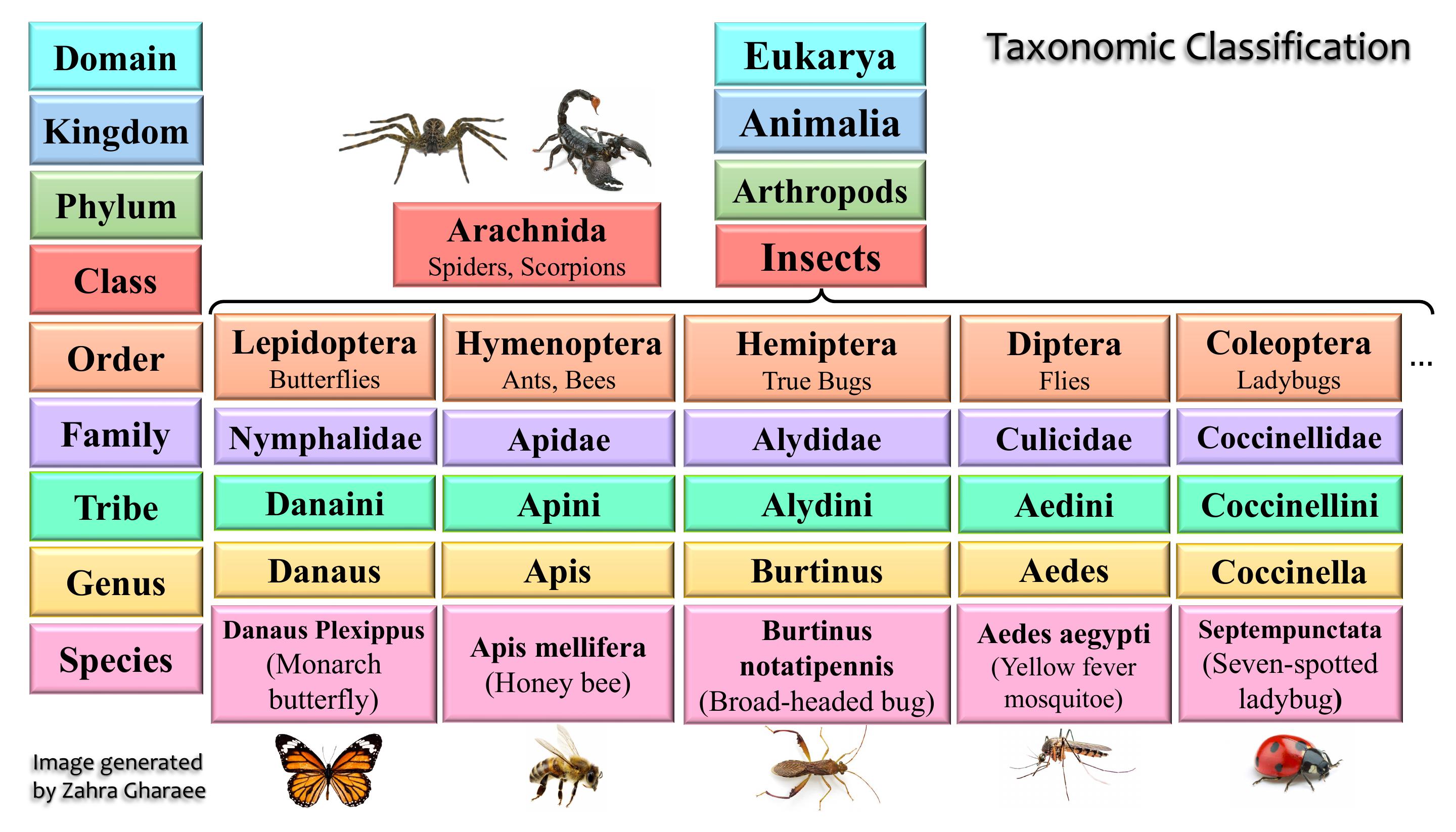
Taxonomic group ranking annotations categorize organisms hierarchically based on evolutionary relationships.
Each dataset sample includes geographic information about the collection sites, captured through four key data attributes:
Each dataset sample includes size information about each specimen, captured through three key data attributes:
Count of pixels occupied by the organism in its image.
The fraction of the original image that the cropped image comprises based on bounding box information.
The ratio of the cropped image to the cropped and resized image based on bounding box information.
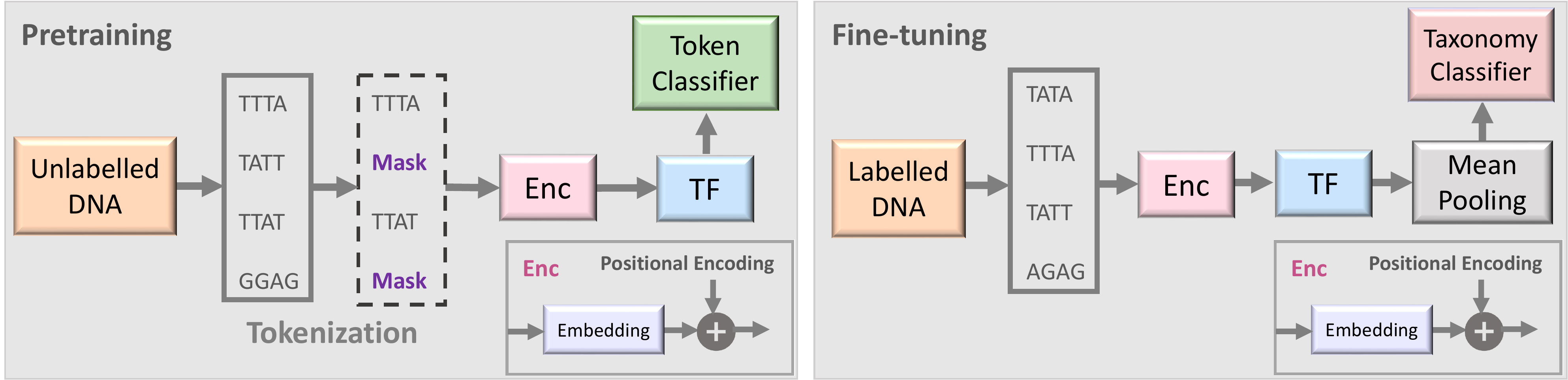
Two stages of the proposed semi-supervised learning set-up based on BarcodeBERT Arias et al. (2023). (1) Pretraining: DNA sequences are tokenized using non-overlapping k-mers and 50% of the tokens are masked for the MLM task. Tokens are encoded and fed into a transformer model. The output embeddings are used for token-level classification. (2) Fine-tuning: All DNA sequences in a dataset are tokenized using non-overlapping k-mer tokenization and all tokenized sequences, without masking, are passed through the pretrained transformer model. Global mean-pooling is applied over the token-level embeddings and the output is used for taxonomic classification.
The results are presented in Gharaee et al. (2024)
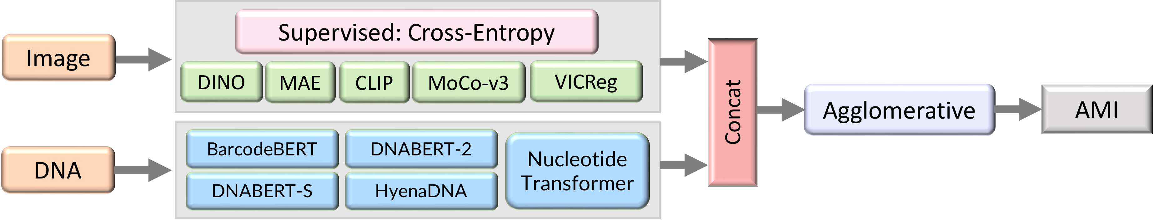
Images and DNA are each passed through one of several pretrained encoders. These representations are clustered with Agglomerative Clustering.
The results are presented in Gharaee et al. (2024)
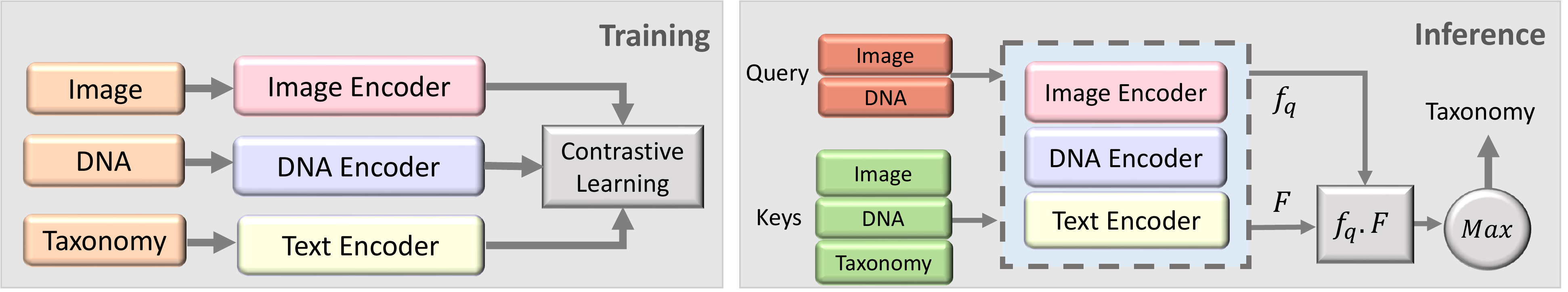
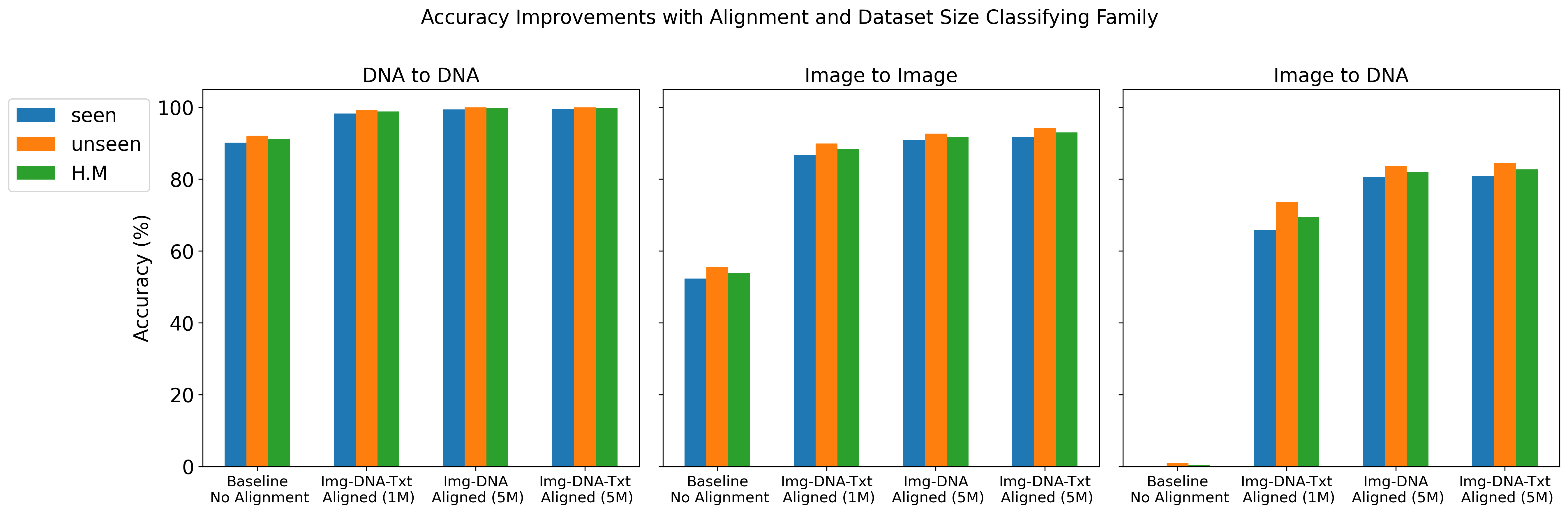
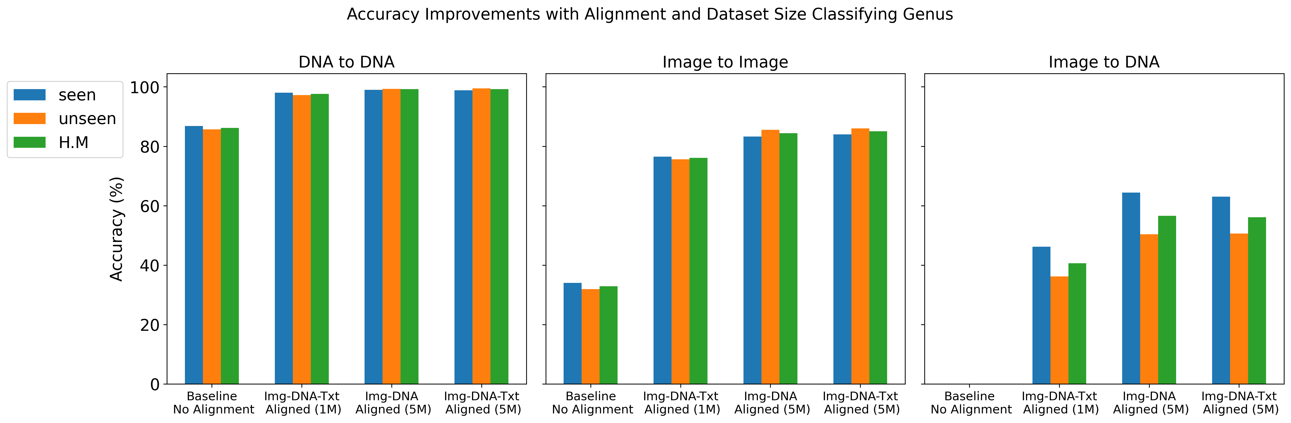
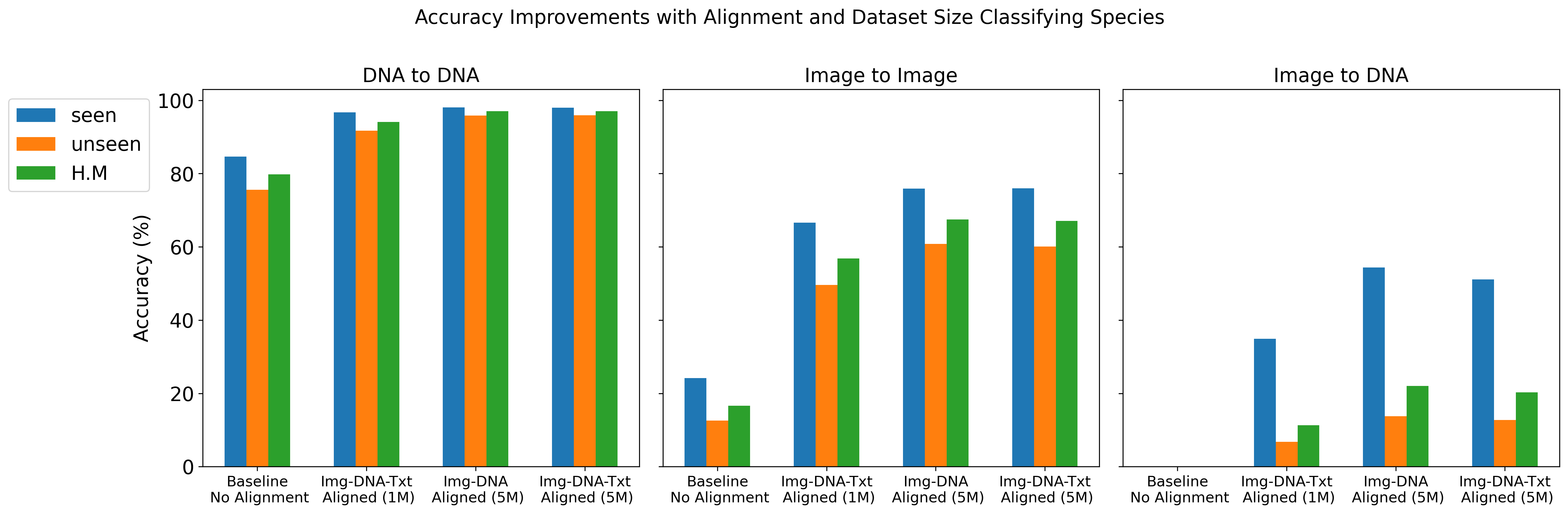
Our experiments using the BIOSCAN-CLIBD Gong et al. (2024) are conducted in two steps. (1) Training: Multiple modalities, including RGB images, textual taxonomy, and DNA sequences, are encoded separately, and trained using a contrastive loss function. (2) Inference: Image vs DNA embedding is used as a query, and compared to the embeddings obtained from a database of image, DNA and text (keys). The cosine similarity is used to find the closest key embedding, and the corresponding taxonomic label is used to classify the query.
We report top-1 macro accuracy (%) on the test set using different amounts of pre-training data (1 million vs. 5 million records from BIOSCAN-5M) and various combinations of aligned embeddings (image, DNA, and text) during contrastive training. Our results include accuracy for image-to-image, DNA-to-DNA, and image-to-DNA query-key combinations. As a baseline, we provide the results without contrastive learning (no alignment). We report accuracy separately for seen and unseen species, along with the harmonic mean (H.M.) between these values.
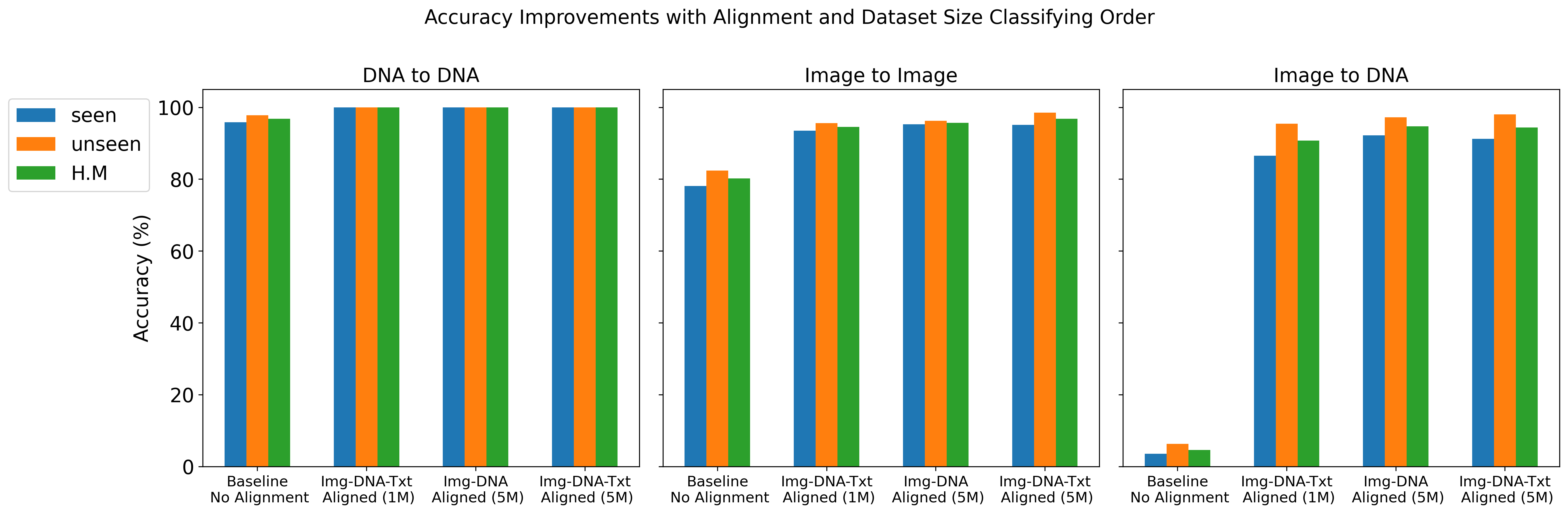
The results details are presented in Gharaee et al. (2024)